Putting it together
Last updated on 2022-11-29 | Edit this page
Overview
Questions
- How do you apply data manipulation skills to multiple new files?
Objectives
- Read in messy data and find issues.
- Replace incorrect values.
- Read data from multiple file formats.
- Utilize
pivot_functions to reshape untidy data. - Combine multiple datasets.
- Understand the process of formatting new data similarly to existing data.
R
library(tidyverse)
So far we have been working with surveys data from 1977 to 1989, and our data have been pretty neat and tidy. There are some NA values, but for the most part, the data have been formatted nicely. However, as many of us know, we do not always receive data in such nice shape. It’s pretty common to get data with all sorts of formatting issues, maybe some strange file formats, and possibly spread across several different sources.
Well, it turns out we have just that situation! We have received a newer batch of surveys data, from 1990 to 2002, and we want to add it to our older dataset so we can work with them together. Unfortunately, the data are not formatted quite as nicely as our old data. Our collaborators have told us to “look them over” for any errors, but have not given us very much specific information. We will have to explore the new data to make sure we understand it and verify that there aren’t any errors.
You can download a .zip file containing three new data files here: https://www.michaelc-m.com/Rewrite-R-ecology-lesson/data/new_data.zip. When prompted, save the file to your data/raw/ folder. A .zip file is a type of compressed file that contains one or more files or directories. We will use the unzip() command to extract the data files from the .zip file. The first argument is the path to the .zip file, the next argument is the directory we want to put the extracted files into, and the last argument tells unzip() to not create an additional directory for the new files. Since this is an action we only want to perform once, we will run it directly in the Console instead of putting it into a script.
R
unzip("data/raw/new_data.zip", exdir = "data/raw/", junkpaths = TRUE)
Use the Files pane in the lower right to navigate to the data/raw/ folder and you should find 3 new files: plots_new.csv, species_new.txt, and surveys_new.csv.
Reading the new surveys data
Let’s start off with the new surveys data. First we will read it into R:
R
surveys_new <- read_csv("data/raw/surveys_new.csv")
WARNING
Warning: One or more parsing issues, see `problems()` for detailsOUTPUT
Rows: 18676 Columns: 7
── Column specification ────────────────────────────────────────────────────────
Delimiter: ","
chr (3): date (mm/dd/yyyy), species_id, sex
dbl (4): record_id, plot_id, hindfoot_length, weight

ℹ Use `spec()` to retrieve the full column specification for this data.
ℹ Specify the column types or set `show_col_types = FALSE` to quiet this message.
You will notice it contains a lot of columns from our previous surveys data, but not all of the columns. Some of them are only found in our other plots_new.csv and species_new.txt files.
First thing we want to do with surveys_new is fix that date column name with spaces in it. R can handle them, but they are often very annoying. We can use the rename() function to change the column name.
R
surveys_new <- surveys_new %>%
  rename(date = `date (mm/dd/yyyy)`)
Let’s take a look at a summary of our data using summary().
R
summary(surveys_new)
OUTPUT
   record_id         date              plot_id       species_id
 Min.   :16879   Length:18676       Min.   : 1.00   Length:18676
 1st Qu.:21545   Class :character   1st Qu.: 5.00   Class :character
 Median :26214   Mode  :character   Median :12.00   Mode  :character
 Mean   :26214                      Mean   :11.33
 3rd Qu.:30881                      3rd Qu.:17.00
 Max.   :35549                      Max.   :24.00

     sex            hindfoot_length     weight
 Length:18676       Min.   : 2.00   Min.   :   4.0
 Class :character   1st Qu.:21.00   1st Qu.:  19.0
 Mode  :character   Median :26.00   Median :  32.0
                    Mean   :27.08   Mean   : 873.7
                    3rd Qu.:36.00   3rd Qu.:  47.0
                    Max.   :64.00   Max.   :9999.0
                    NA's   :1380
The summary() function is often useful for detecting outliers or clearly incorrect values, since we get a Min. and Max. value for each numeric column. For example, we see that month goes from 1 to 12 and day goes from 1 to 31, so no issues there. However, we do notice that weight has a max value of 9999. Sometimes people will use extreme and impossible values to denote a missing value. It is worth checking with our collaborators to make sure this is the case, but we will assume that’s what happened.
Finally, we actually got a warning message about a parsing issue. This message actually comes from read_csv(), even though it only showed up now. Parsing is what read_csv() does when it tries to guess what type of vector each CSV column should be. Sometimes it will warn us about issues that occurred, which we can then investigate with the problems() function.
R
problems(surveys_new)
OUTPUT
# A tibble: 1 × 5
    row   col expected actual file
  <int> <int> <chr>    <chr>  <chr>
1    19     6 a double 19'    /home/runner/work/Rewrite-R-ecology-lesson/Rewrit…
The output shows that in the 19th row and 8th column of the CSV, read_csv() expected a double, or numeric, value. Instead, what it got was 19'. That stray quotation mark was unexpected, so read_csv() notified us. Let’s go see what value is actually there for surveys_new. It was in the 19th row of the CSV, which includes the header row containing column names, so we should look at the 18th row of our data.frame. The 8th column is hindfoot_length. We can use the head() function to look at the first 20 rows.
R
surveys_new %>%
  head(n=20)
OUTPUT
# A tibble: 20 × 7
   record_id date     plot_id species_id sex   hindfoot_length weight
       <dbl> <chr>      <dbl> <chr>      <chr>           <dbl>  <dbl>
 1     16879 1/6/1990       1 DM         F                  37     35
 2     16880 1/6/1990       1 OL         M                  21     28
 3     16881 1/6/1990       6 PF         M                  16      7
 4     16882 1/6/1990      23 RM         F                  17      9
 5     16883 1/6/1990      12 RM         M                  17     10
 6     16884 1/6/1990      24 RM         M                  17      9
 7     16885 1/6/1990      12 SF         M                  25     35
 8     16886 1/6/1990      24 SH         F                  30     73
 9     16887 1/6/1990      12 SF         M                  28     44
10     16888 1/6/1990      17 DO         M                  36     55
11     16889 1/6/1990      21 SF         M                  29     55
12     16890 1/6/1990      12 OT         M                  22     23
13     16891 1/6/1990      12 DO         F                  36     53
14     16892 1/6/1990      21 AB         <NA>               NA   9999
15     16893 1/6/1990      12 OT         F                  21     24
16     16894 1/6/1990       1 OT         F                  21     20
17     16895 1/6/1990      12 SF         F                  27     75
18     16896 1/6/1990      12 RM         M                  NA     11
19     16897 1/6/1990      21 SF         F                  29     46
20     16898 1/6/1990      23 RM         M                  18     11
Because read_csv() didn’t know what to do with the value 19', there is an NA for hindfoot_length in row 18. It is likely that the true value was 19 and the stray quotation mark was simply a typo. If we want to change that value, we can do it by referring to the record_id, since it is a unique identifier for each row. We will use the function if_else() to actually replace the value. This function takes a logical statement as its first argument, then a value to return if that statement is TRUE, and a value to return if it is FALSE. Take a look at this example:
R
x <- 1:10
ifelse(x > 6, "bigger than 6", "not bigger than 6")
OUTPUT
 [1] "not bigger than 6" "not bigger than 6" "not bigger than 6"
 [4] "not bigger than 6" "not bigger than 6" "not bigger than 6"
 [7] "bigger than 6"     "bigger than 6"     "bigger than 6"
[10] "bigger than 6"
What we will do is take surveys_new and mutate the hindfoot_length column. It will be equal to the result of an ifelse() statement. If the record_id is 16896, the row we are trying to change, then hindfoot_length will be set to 19. If the record_id is not 16896, then it will stay as the current hindfoot_length value.
R
surveys_new <- surveys_new %>%
  mutate(hindfoot_length = ifelse(record_id == 16896, 19, hindfoot_length))

surveys_new %>%
  head(n=20)
OUTPUT
# A tibble: 20 × 7
   record_id date     plot_id species_id sex   hindfoot_length weight
       <dbl> <chr>      <dbl> <chr>      <chr>           <dbl>  <dbl>
 1     16879 1/6/1990       1 DM         F                  37     35
 2     16880 1/6/1990       1 OL         M                  21     28
 3     16881 1/6/1990       6 PF         M                  16      7
 4     16882 1/6/1990      23 RM         F                  17      9
 5     16883 1/6/1990      12 RM         M                  17     10
 6     16884 1/6/1990      24 RM         M                  17      9
 7     16885 1/6/1990      12 SF         M                  25     35
 8     16886 1/6/1990      24 SH         F                  30     73
 9     16887 1/6/1990      12 SF         M                  28     44
10     16888 1/6/1990      17 DO         M                  36     55
11     16889 1/6/1990      21 SF         M                  29     55
12     16890 1/6/1990      12 OT         M                  22     23
13     16891 1/6/1990      12 DO         F                  36     53
14     16892 1/6/1990      21 AB         <NA>               NA   9999
15     16893 1/6/1990      12 OT         F                  21     24
16     16894 1/6/1990       1 OT         F                  21     20
17     16895 1/6/1990      12 SF         F                  27     75
18     16896 1/6/1990      12 RM         M                  19     11
19     16897 1/6/1990      21 SF         F                  29     46
20     16898 1/6/1990      23 RM         M                  18     11
We can actually use ifelse() to fix the values of 9999 in the weight column as well.
R
surveys_new <- surveys_new %>%
  mutate(weight = ifelse(weight == 9999, NA, weight))

surveys_new %>%
  head(n=20)
OUTPUT
# A tibble: 20 × 7
   record_id date     plot_id species_id sex   hindfoot_length weight
       <dbl> <chr>      <dbl> <chr>      <chr>           <dbl>  <dbl>
 1     16879 1/6/1990       1 DM         F                  37     35
 2     16880 1/6/1990       1 OL         M                  21     28
 3     16881 1/6/1990       6 PF         M                  16      7
 4     16882 1/6/1990      23 RM         F                  17      9
 5     16883 1/6/1990      12 RM         M                  17     10
 6     16884 1/6/1990      24 RM         M                  17      9
 7     16885 1/6/1990      12 SF         M                  25     35
 8     16886 1/6/1990      24 SH         F                  30     73
 9     16887 1/6/1990      12 SF         M                  28     44
10     16888 1/6/1990      17 DO         M                  36     55
11     16889 1/6/1990      21 SF         M                  29     55
12     16890 1/6/1990      12 OT         M                  22     23
13     16891 1/6/1990      12 DO         F                  36     53
14     16892 1/6/1990      21 AB         <NA>               NA     NA
15     16893 1/6/1990      12 OT         F                  21     24
16     16894 1/6/1990       1 OT         F                  21     20
17     16895 1/6/1990      12 SF         F                  27     75
18     16896 1/6/1990      12 RM         M                  19     11
19     16897 1/6/1990      21 SF         F                  29     46
20     16898 1/6/1990      23 RM         M                  18     11
Challenge 1: Find a specialized function
The tidyverse often has specialized functions for common data manipulation tasks, such as replacing a certain values with NA. There is a tidyverse function to replace a value in a vector with NA. Put your Googling skills to work and see if you can find the correct function.
For an extra challenge, write out code that could use this function to replace weight values of 9999 with NA.
The dplyr function na_if() will replace specific values in a vector to NA. To find this function, you can Google “tidyverse replace value with NA”. One of the first results is the dplyr documentation page for the na_if() function.
If you scroll down to the bottom section of the documentation, you will find several examples, including how to use the function inside mutate().
R
surveys_new %>%
  mutate(weight = na_if(weight, 9999))
The last thing we have to do is deal with our date column. It’s currently a character column, but our old surveys data had separate columns for year, month, and day. Another thing we should do is check for any errors in our dates, since they are an error-prone data type.
There are a few ways we could approach this problem, which is a common theme in R: there are often many ways to accomplish the same task. It is often useful to plan your approach ahead of time, so we will describe two possible methods:
Turn the current column into a date column, validate the dates, then use
lubridatefunctions to extract the year, month, and day into their own columns.Use the
separate()function to split our current date column into 3 new character columns, containing the month, day and year. Then turn those columns into numeric columns. Then it will match our oldsurveysdata, and we can later make a date column to validate our dates.
It is often useful to plan out your approach, or several approaches, before you start writing code. It can be in the form of plain English like above, or in “pseudo-code”, which is laid out like code, but doesn’t have explicit, functioning code.
We will go ahead and use the first approach. First we will load lubridate and use the mdy() function to turn our date column into a date instead of character column.
R
library(lubridate)
OUTPUT
Attaching package: 'lubridate'OUTPUT
The following objects are masked from 'package:base':

    date, intersect, setdiff, union
R
surveys_new <- surveys_new %>%
  mutate(date = mdy(date))
WARNING
Warning: 6 failed to parse.We got a warning message about 6 dates failing to parse. This means that the mdy() function encountered 6 dates that it wasn’t able to identify correctly. When lubridate functions fail to parse dates, they will return an NA value instead. To find the rows where this happened, we can use filter():
R
surveys_new %>%
  filter(is.na(date))
OUTPUT
# A tibble: 6 × 7
  record_id date   plot_id species_id sex   hindfoot_length weight
      <dbl> <date>   <dbl> <chr>      <chr>           <dbl>  <dbl>
1     22258 NA           8 AH         <NA>               NA     NA
2     22261 NA           9 DM         F                  37     45
3     30595 NA          18 PB         F                  25     34
4     30610 NA           2 PB         F                  25     31
5     30638 NA          20 PP         F                  22     20
6     31394 NA          12 OT         F                  20     29
Challenge 2: Find the bad dates
We have now located the rows with NA dates, but we probably want to know what the original date character strings looked like. Figure out what those dates were and why they might have been wrong.
Hint: you will have to look at a previous version of the data, before we modified the date column.
There are two basic approaches you could take. First, you could look directly at the old CSV and find the rows with bad dates based on their record_id.
You could also read the data back into R and use filter() to pick out those specific rows via record_id:
R
read_csv("data/raw/surveys_new.csv") %>%
  filter(record_id %in% c(22258, 22261, 30595, 30610, 30638, 31394))
WARNING
Warning: One or more parsing issues, see `problems()` for detailsOUTPUT
# A tibble: 6 × 7
  record_id `date (mm/dd/yyyy)` plot_id species_id sex   hindfoot_length weight
      <dbl> <chr>                 <dbl> <chr>      <chr>           <dbl>  <dbl>
1     22258 4/31/1995                 8 AH         <NA>               NA   9999
2     22261 4/31/1995                 9 DM         F                  37     45
3     30595 4/31/2000                18 PB         F                  25     34
4     30610 4/31/2000                 2 PB         F                  25     31
5     30638 4/31/2000                20 PP         F                  22     20
6     31394 9/31/2000                12 OT         F                  20     29
The dates are wrong because they are the 31st day in a month that only has 30 days, like April or September. lubridate doesn’t recognize these as valid dates. The same thing can happen with things like dates in February during non-leap years.
The last thing to do is extract the year, month, and day values from our date column. lubridate has functions to extract each component of a date. We will then get rid of the date column, since it doesn’t appear in our original surveys data, and we can always remake it from the component columns.
R
surveys_new <- surveys_new %>%
  mutate(year = year(date),
         month = month(date),
         day = day(date)) %>%
  select(-date)

surveys_new
OUTPUT
# A tibble: 18,676 × 9
   record_id plot_id species_id sex   hindfoot_length weight  year month   day
       <dbl>   <dbl> <chr>      <chr>           <dbl>  <dbl> <dbl> <dbl> <int>
 1     16879       1 DM         F                  37     35  1990     1     6
 2     16880       1 OL         M                  21     28  1990     1     6
 3     16881       6 PF         M                  16      7  1990     1     6
 4     16882      23 RM         F                  17      9  1990     1     6
 5     16883      12 RM         M                  17     10  1990     1     6
 6     16884      24 RM         M                  17      9  1990     1     6
 7     16885      12 SF         M                  25     35  1990     1     6
 8     16886      24 SH         F                  30     73  1990     1     6
 9     16887      12 SF         M                  28     44  1990     1     6
10     16888      17 DO         M                  36     55  1990     1     6
# … with 18,666 more rows
Reading the new species data
Our surveys_new data look good at this point, so let’s move on to the species data. You may have noticed that our species data came in a different file format, species_new.txt. So far we have been working with CSV files, in which values are separated by commas. However, R is capable of reading many different file types. The .txt extension means it is a plain-text file, which means the data could be formatted in quite a few different ways. Let’s take a look at the file directly to see how it is structured.
Click on the species_new.txt file in the Files pane to open it in RStudio. We see that our data are still structured in columns and rows, with column names in the header row. Each value is wrapped in quotes, values are separated by spaces, and each row ends with a new line.
This is a generic data structure called “delimited” data. A CSV is a form of delimited data, where values are “delimited”, or separated, by commas. Luckily, the readr package has a function for dealing with more generic delimited data, called read_delim().
We have to give read_delim() three arguments. First is the file path, just like read_csv(). The second argument is what character string is used to delimit each item in the file. In our case, it is a space, so we make a character string that is just a space. Finally, we need to identify what is used to quote each entry in our file. Our values are wrapped in double-quotes, so we need to type a double quote. However, we can’t just type 3 double-quotes, or R will get upset with us (give it a try if you want). Luckily, R recognizes both single- and double-quotes for creating character strings. So we can use single-quotes to make our character string, and put one double-quote character inside it.
R
species_new <- read_delim("data/raw/species_new.txt", delim = " ", quote = '"')
OUTPUT
Rows: 54 Columns: 3
── Column specification ────────────────────────────────────────────────────────
Delimiter: " "
chr (3): species_id, species_name, taxa

ℹ Use `spec()` to retrieve the full column specification for this data.
ℹ Specify the column types or set `show_col_types = FALSE` to quiet this message.
R
species_new
OUTPUT
# A tibble: 54 × 3
   species_id species_name                    taxa
   <chr>      <chr>                           <chr>
 1 AB         Amphispiza bilineata            Bird
 2 AH         Ammospermophilus harrisi        Rodent
 3 AS         Ammodramus savannarum           Bird
 4 BA         Baiomys taylori                 Rodent
 5 CB         Campylorhynchus brunneicapillus Bird
 6 CM         Calamospiza melanocorys         Bird
 7 CQ         Callipepla squamata             Bird
 8 CS         Crotalus scutalatus             Reptile
 9 CT         Cnemidophorus tigris            Reptile
10 CU         Cnemidophorus uniparens         Reptile
# … with 44 more rows
What we get back is a tibble, formatted just like it would have been if our data were in a CSV.
One thing we might notice is that our species and genus are combined into one column called species_name, whereas in our old data, we had separate columns for genus and species. It is fairly common to have data in one column that could be separated into two or more columns. Luckily, tidyr has a convenient function for solving this problem, called separate().
We pipe species_new into the separate() function, then give it several other arguments. First, the name of the column to be separated, species_name. Next, we give the argument into a character vector of the new columns we want. Finally, we give a string for what is currently separating each of the new values in the current column. In species_name, the genus and species are separated by a space.
R
species_new <- species_new %>%
  separate(species_name, into = c("genus", "species"), sep = " ")

species_new
OUTPUT
# A tibble: 54 × 4
   species_id genus            species         taxa
   <chr>      <chr>            <chr>           <chr>
 1 AB         Amphispiza       bilineata       Bird
 2 AH         Ammospermophilus harrisi         Rodent
 3 AS         Ammodramus       savannarum      Bird
 4 BA         Baiomys          taylori         Rodent
 5 CB         Campylorhynchus  brunneicapillus Bird
 6 CM         Calamospiza      melanocorys     Bird
 7 CQ         Callipepla       squamata        Bird
 8 CS         Crotalus         scutalatus      Reptile
 9 CT         Cnemidophorus    tigris          Reptile
10 CU         Cnemidophorus    uniparens       Reptile
# … with 44 more rows
There we go, now species_new is formatted like the similar columns in the older surveys data.
The separate() function also has an argument called convert, which will automatically convert the types of your new columns. For example, if you had a column called range that had character strings like "1990-1995", and you wanted to separate it into start and end columns, you would end up with character columns if you used separate() like we did above. However, if you use convert = T, the new columns will be converted to integers. Check out this short example below:
R
d <- tibble(years = c("1990-1995", "2000-2002"))

d %>%
  separate(years, into = c("start", "end"), sep = "-")
OUTPUT
# A tibble: 2 × 2
  start end
  <chr> <chr>
1 1990  1995
2 2000  2002
R
d %>%
  separate(years, into = c("start", "end"), sep = "-", convert = T)
OUTPUT
# A tibble: 2 × 2
  start   end
  <int> <int>
1  1990  1995
2  2000  2002
Reading the new plots data
Finally, we can move on to the new plots data, in the plots_new.csv file. We can go back to read_csv() to get it into R.
R
plots_new <- read_csv("data/raw/plots_new.csv")
OUTPUT
Rows: 1 Columns: 24
── Column specification ────────────────────────────────────────────────────────
Delimiter: ","
chr (24): Plot 1, Plot 2, Plot 3, Plot 4, Plot 5, Plot 6, Plot 7, Plot 8, Pl...

ℹ Use `spec()` to retrieve the full column specification for this data.
ℹ Specify the column types or set `show_col_types = FALSE` to quiet this message.
R
plots_new
OUTPUT
# A tibble: 1 × 24
  `Plot 1`        `Plot 2` `Plot 3` `Plot 4` `Plot 5` `Plot 6` `Plot 7` `Plot 8`
  <chr>           <chr>    <chr>    <chr>    <chr>    <chr>    <chr>    <chr>
1 Spectab exclos… Control  Long-te… Control  Rodent … Short-t… Rodent … Control
# … with 16 more variables: `Plot 9` <chr>, `Plot 10` <chr>, `Plot 11` <chr>,
#   `Plot 12` <chr>, `Plot 13` <chr>, `Plot 14` <chr>, `Plot 15` <chr>,
#   `Plot 16` <chr>, `Plot 17` <chr>, `Plot 18` <chr>, `Plot 19` <chr>,
#   `Plot 20` <chr>, `Plot 21` <chr>, `Plot 22` <chr>, `Plot 23` <chr>,
#   `Plot 24` <chr>
It looks like our data are in a bit of a strange format. We have a column for each plot, and then a single row of data containing the plot type. If you look at our old surveys data, we had a single row for plot_id and a single row for plot_type. surveys contained this data in a long format, whereas plots_new has a wide format.
R
plots_new <- plots_new %>%
  pivot_longer(cols = everything(), names_to = "plot_id", values_to = "plot_type")

plots_new
OUTPUT
# A tibble: 24 × 2
   plot_id plot_type
   <chr>   <chr>
 1 Plot 1  Spectab exclosure
 2 Plot 2  Control
 3 Plot 3  Long-term Krat Exclosure
 4 Plot 4  Control
 5 Plot 5  Rodent Exclosure
 6 Plot 6  Short-term Krat Exclosure
 7 Plot 7  Rodent Exclosure
 8 Plot 8  Control
 9 Plot 9  Spectab exclosure
10 Plot 10 Rodent Exclosure
# … with 14 more rows
Our old surveys data had plot_id as a numeric variable, but ours is a character string with "Plot " in front of the number. This is a pretty common issue, but we can use a function from the stringr package to fix it.
We will use mutate() to modify the plot_id column, and we will replace it with the results of the str_replace() function. The first argument to str_replace() is the character vector we want to modify, which is the current plot_id column. Next is the string of characters that we want to replace, which is "Plot ", including the space at the end. Finally, we have the replacement string. Since we want to remove "Plot ", we replace it with a blank string "".
R
plots_new <- plots_new %>%
  mutate(plot_id = str_replace(plot_id, "Plot ", ""))

plots_new
OUTPUT
# A tibble: 24 × 2
   plot_id plot_type
   <chr>   <chr>
 1 1       Spectab exclosure
 2 2       Control
 3 3       Long-term Krat Exclosure
 4 4       Control
 5 5       Rodent Exclosure
 6 6       Short-term Krat Exclosure
 7 7       Rodent Exclosure
 8 8       Control
 9 9       Spectab exclosure
10 10      Rodent Exclosure
# … with 14 more rows
We successfully removed "Plot " from our plot_id column entries, so we are left with just the numbers. However, it is still a character column. The last step is to convert it to a numeric column.
R
plots_new <- plots_new %>%
  mutate(plot_id = as.numeric(plot_id))

plots_new
OUTPUT
# A tibble: 24 × 2
   plot_id plot_type
     <dbl> <chr>
 1       1 Spectab exclosure
 2       2 Control
 3       3 Long-term Krat Exclosure
 4       4 Control
 5       5 Rodent Exclosure
 6       6 Short-term Krat Exclosure
 7       7 Rodent Exclosure
 8       8 Control
 9       9 Spectab exclosure
10      10 Rodent Exclosure
# … with 14 more rows
Joining the new data
Now that we have each individual data.frame formatted nicely, we would like to be able to combine them. Our surveys data has all of the data combined into one data.frame. However, our data.frames are different sizes. surveys_new has 18676 rows, and it contains the individual data for each animal. This is the same basic size of the old surveys data. However, our plots_new and species_new data are much smaller. They only contain data on specific plots and species.
If we look at the column names for surveys_new and plots_new, we see that they share a plot_id column. What we want to do now is take the data of our actual observations, surveys_new, and add the data for each associated plot. If a row in surveys_new has a plot_id of 2, we want to associate the plot_type of that plot with that row. We can accomplish this using a join.
There are several types of joins in the dplyr package, which you can read more about here. We will use a function called left_join(), which takes two dataframes and adds the columns from the second dataframe to the first dataframe, matching rows based on the column name supplied to the by argument.
R
left_join(surveys_new, plots_new, by = "plot_id")
OUTPUT
# A tibble: 18,676 × 10
   record_id plot_id species_id sex   hindfoot_length weight  year month   day
       <dbl>   <dbl> <chr>      <chr>           <dbl>  <dbl> <dbl> <dbl> <int>
 1     16879       1 DM         F                  37     35  1990     1     6
 2     16880       1 OL         M                  21     28  1990     1     6
 3     16881       6 PF         M                  16      7  1990     1     6
 4     16882      23 RM         F                  17      9  1990     1     6
 5     16883      12 RM         M                  17     10  1990     1     6
 6     16884      24 RM         M                  17      9  1990     1     6
 7     16885      12 SF         M                  25     35  1990     1     6
 8     16886      24 SH         F                  30     73  1990     1     6
 9     16887      12 SF         M                  28     44  1990     1     6
10     16888      17 DO         M                  36     55  1990     1     6
# … with 18,666 more rows, and 1 more variable: plot_type <chr>
Now we have our surveys_new dataframe, still with 18676 rows, but now each row has a value for plot_type, corresponding to its entry in plot_id. We can assign this back to surveys_new, so that it now contains the information from both dataframes.
R
surveys_new <- left_join(surveys_new, plots_new, by = "plot_id")
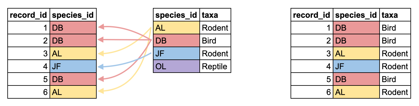
We can repeat this process to get the information from species_new. surveys_new and species_new both have a species_id column, but we would like to add the genus, species, and taxa information to surveys_new.
R
surveys_new <- left_join(surveys_new, species_new, by = "species_id")

surveys_new
OUTPUT
# A tibble: 18,676 × 13
   record_id plot_id species_id sex   hindfoot_length weight  year month   day
       <dbl>   <dbl> <chr>      <chr>           <dbl>  <dbl> <dbl> <dbl> <int>
 1     16879       1 DM         F                  37     35  1990     1     6
 2     16880       1 OL         M                  21     28  1990     1     6
 3     16881       6 PF         M                  16      7  1990     1     6
 4     16882      23 RM         F                  17      9  1990     1     6
 5     16883      12 RM         M                  17     10  1990     1     6
 6     16884      24 RM         M                  17      9  1990     1     6
 7     16885      12 SF         M                  25     35  1990     1     6
 8     16886      24 SH         F                  30     73  1990     1     6
 9     16887      12 SF         M                  28     44  1990     1     6
10     16888      17 DO         M                  36     55  1990     1     6
# … with 18,666 more rows, and 4 more variables: plot_type <chr>, genus <chr>,
#   species <chr>, taxa <chr>
Now our surveys_new dataframe has all the information from our 3 files, and the same number of columns as our original surveys data.
Adding to the old data
Now that our old surveys data and surveys_new data are formatted in the same way, we can bind them together so we have data from all years in one data.frame. First let’s read our `surveys’ data back in.
R
surveys <- read_csv("data/cleaned/surveys_complete_77_89.csv")
OUTPUT
Rows: 16878 Columns: 13
── Column specification ────────────────────────────────────────────────────────
Delimiter: ","
chr (6): species_id, sex, genus, species, taxa, plot_type
dbl (7): record_id, month, day, year, plot_id, hindfoot_length, weight

ℹ Use `spec()` to retrieve the full column specification for this data.
ℹ Specify the column types or set `show_col_types = FALSE` to quiet this message.
Now we can use the bind_rows() function to bind the rows of our two data.frames together. The fact that our columns are not in the same order doesn’t matter, bind_rows() will detect thatt the column names are the same, and will rearrange them to match the first data.frame.
R
surveys_complete <- bind_rows(surveys, surveys_new)

surveys_complete
OUTPUT
# A tibble: 35,554 × 13
   record_id month   day  year plot_id species_id sex   hindfoot_length weight
       <dbl> <dbl> <dbl> <dbl>   <dbl> <chr>      <chr>           <dbl>  <dbl>
 1         1     7    16  1977       2 NL         M                  32     NA
 2         2     7    16  1977       3 NL         M                  33     NA
 3         3     7    16  1977       2 DM         F                  37     NA
 4         4     7    16  1977       7 DM         M                  36     NA
 5         5     7    16  1977       3 DM         M                  35     NA
 6         6     7    16  1977       1 PF         M                  14     NA
 7         7     7    16  1977       2 PE         F                  NA     NA
 8         8     7    16  1977       1 DM         M                  37     NA
 9         9     7    16  1977       1 DM         F                  34     NA
10        10     7    16  1977       6 PF         F                  20     NA
# … with 35,544 more rows, and 4 more variables: genus <chr>, species <chr>,
#   taxa <chr>, plot_type <chr>
We might be interested in indicating which rows of our data came from which source: the old data or the new. We can name the data.frames inside bind_rows(), and then give a new argument .id. This will give us a new column called source that contains a value of "old" for rows that came from surveys, and a value of "new" for rows that came from surveys_new.
R
surveys_complete <- bind_rows(old = surveys, new = surveys_new, .id = "source")

surveys_complete
OUTPUT
# A tibble: 35,554 × 14
   source record_id month   day  year plot_id species_id sex   hindfoot_length
   <chr>      <dbl> <dbl> <dbl> <dbl>   <dbl> <chr>      <chr>           <dbl>
 1 old            1     7    16  1977       2 NL         M                  32
 2 old            2     7    16  1977       3 NL         M                  33
 3 old            3     7    16  1977       2 DM         F                  37
 4 old            4     7    16  1977       7 DM         M                  36
 5 old            5     7    16  1977       3 DM         M                  35
 6 old            6     7    16  1977       1 PF         M                  14
 7 old            7     7    16  1977       2 PE         F                  NA
 8 old            8     7    16  1977       1 DM         M                  37
 9 old            9     7    16  1977       1 DM         F                  34
10 old           10     7    16  1977       6 PF         F                  20
# … with 35,544 more rows, and 5 more variables: weight <dbl>, genus <chr>,
#   species <chr>, taxa <chr>, plot_type <chr>
We have now successfully cleaned our new data and reshaped it to match our old data so they could be arranged into one data.frame covering all the years.
Back to ggplot2
position_dodge()-
coord_? patchwork-
label_wrap_gen()? theme_set()
R
surveys_complete %>%
  count(year) %>%
  ggplot(aes(x = year, y = n)) +
  geom_line()
WARNING
Warning: Removed 1 row(s) containing missing values (geom_path).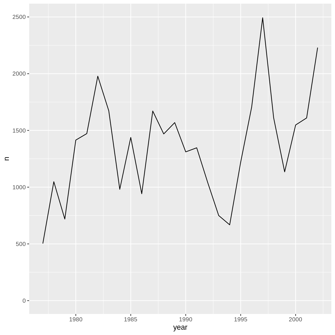
R
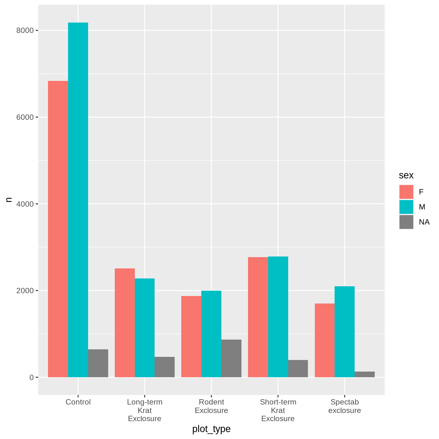
surveys_complete %>%
  count(plot_type, sex) %>%
  ggplot(aes(x = plot_type, y = n, fill = sex)) +
  geom_col(position = position_dodge()) +
  scale_x_discrete(labels = label_wrap_gen(10))
R
surveys_complete %>%
  filter(!is.na(weight), !is.na(sex)) %>%
  group_by(genus, year, sex) %>%
  summarise(mean_weight = mean(weight)) %>%
  ggplot(aes(x = year, y = mean_weight, color = genus)) +
  geom_line() +
  facet_wrap(vars(sex))
OUTPUT
`summarise()` has grouped output by 'genus', 'year'. You can override using the
`.groups` argument.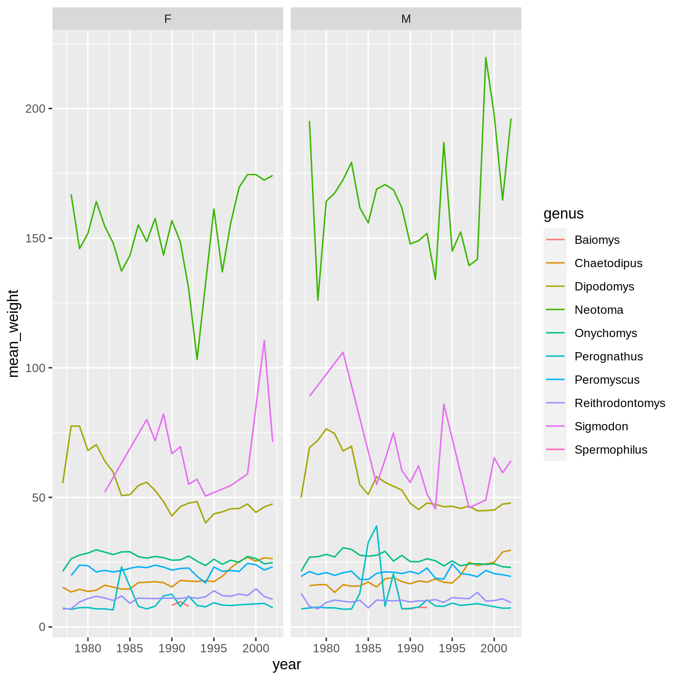
Setting limits with scale_ or xlim()/ylim() will remove data, so the slope of the line changes:
R
surveys_complete %>%
  ggplot(aes(x = weight, y = hindfoot_length)) +
  geom_point() +
  geom_smooth(method = "lm") +
  scale_x_continuous(limits = c(0,100))
OUTPUT
`geom_smooth()` using formula 'y ~ x'WARNING
Warning: Removed 7433 rows containing non-finite values (stat_smooth).WARNING
Warning: Removed 7433 rows containing missing values (geom_point).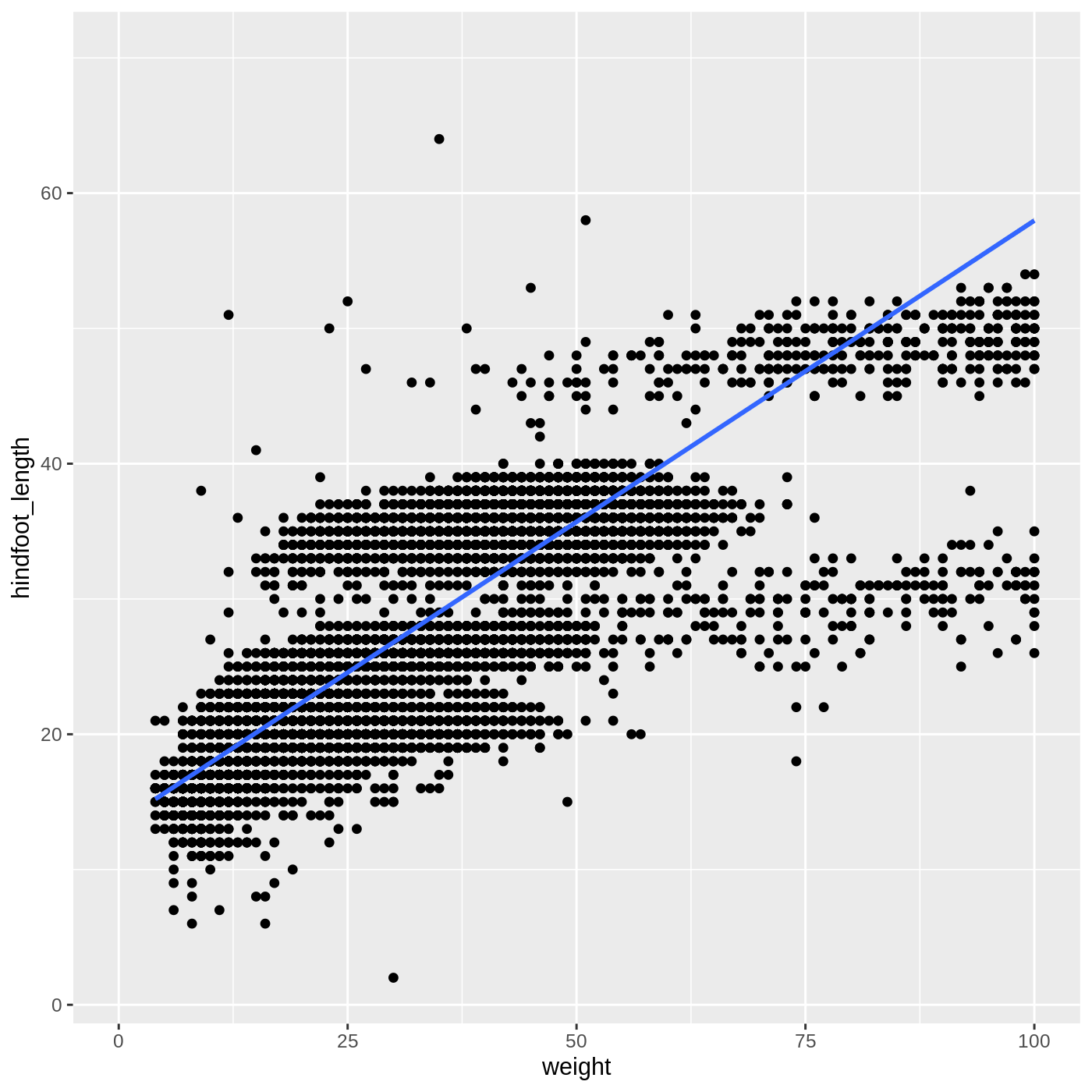
If you want to zoom in on the plot without removing data outside the limits, set the limits inside coord_cartestian():
R
surveys_complete %>%
  ggplot(aes(x = weight, y = hindfoot_length)) +
  geom_point() +
  geom_smooth(method = "lm") +
  coord_cartesian(xlim = c(0,100))
OUTPUT
`geom_smooth()` using formula 'y ~ x'WARNING
Warning: Removed 4812 rows containing non-finite values (stat_smooth).WARNING
Warning: Removed 4812 rows containing missing values (geom_point).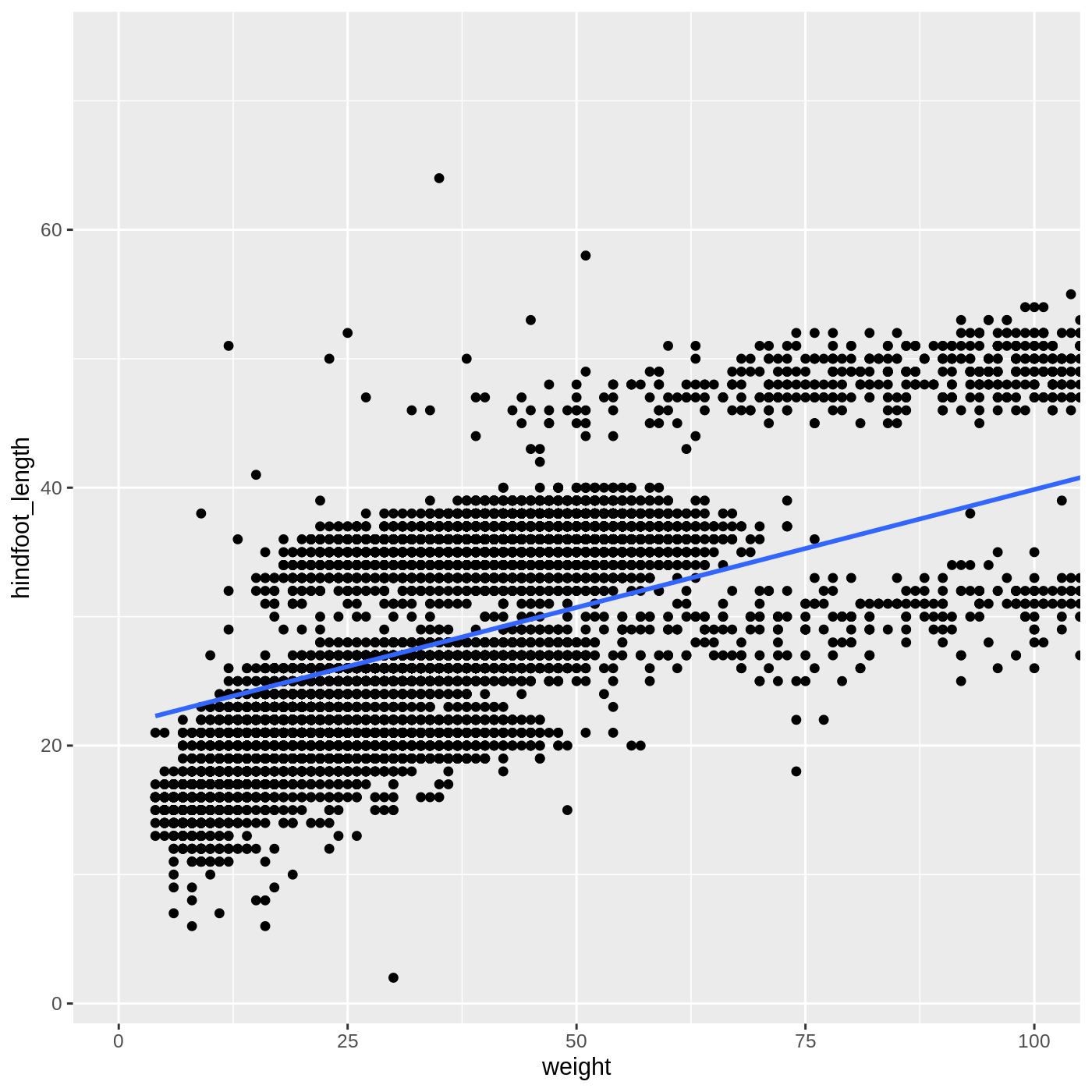
There are other coord_ functions if you need to plot using polar coordinates, map coordinates, or fix the aspect ratio of a plot.
Final outputs
Let’s go ahead and write our data to a CSV file so we can share it with others.
R
surveys_complete %>%
  write_csv("data/cleaned/surveys_complete.csv")
Now we might be interested in looking at all of our data together. Try making some plots of your own to look at the whole dataset!
R
surveys_complete %>%
  ggplot(aes(x = weight, y = hindfoot_length)) +
  geom_point(alpha = 0.05) +
  facet_wrap(vars(source))
WARNING
Warning: Removed 4812 rows containing missing values (geom_point).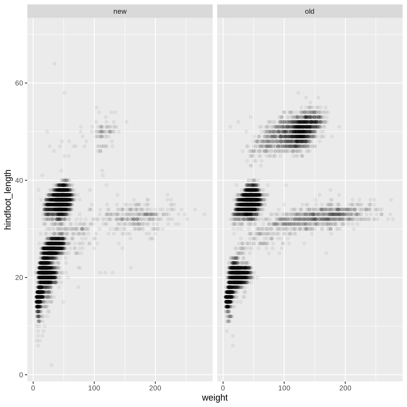
Keypoints
- it is always good to do preliminary investigations of new data
- there are often many ways to achieve the same goal, describing them with plain English or pseudocode can help you choose an approach
- the
read_delimited()function can read tabular data from multiple file formats - joins are powerful ways to combine multiple datasets
- it is a good idea to plan out the steps of your data cleaning and combining