Content from Introduction to R and RStudio
Last updated on 2022-11-29 | Edit this page
Overview
Questions
- Why should you use R and RStudio?
- How do you get started working in R and RStudio?
Objectives
- Understand the difference between R and RStudio
- Describe the purpose of the different RStudio panes
- Organize files and directories into R Projects
- Use the RStudio help interface to get help with R functions
- Be able to format questions to get help in the broader R community
What are R and RStudio?
R refers to a programming language as well as the software that runs R code.
RStudio is a software interface that can make it easier to write R scripts and interact with the R software. It’s a very popular platform, and RStudio also maintains the tidyverse series of packages we will use in this lesson.
Why learn R?
You’re working on a project when your advisor suggests that you begin working with one of their long-time collaborators. According to your advisor, this collaborator is very talented, but only speaks a language that you don’t know. Your advisor assures you that this is ok, the collaborator won’t judge you for starting to learn the language, and will happily answer your questions. However, the collaborator is also quite pedantic. While they don’t mind that you don’t speak their language fluently yet, they are always going to answer you quite literally.
You decide to reach out to the collaborator. You find that they email you back very quickly, almost immediately most of the time. Since you’re just learning their language, you often make mistakes. Sometimes, they tell you that you’ve made a grammatical error or warn you that what you asked for doesn’t make a lot of sense. Sometimes these warnings are difficult to understand, because you don’t really have a grasp of the underlying grammar. Sometimes you get an answer back, with no warnings, but you realize that it doesn’t make sense, because what you asked for isn’t quite what you wanted. Since this collaborator responds almost immediately, without tiring, you can quickly reformulate your question and send it again.
In this way, you begin to learn the language your collaborator speaks, as well as the particular way they think about your work. Eventually, the two of you develop a good working relationship, where you understand how to ask them questions effectively, and how to work through any issues in communication that might arise.
This collaborator’s name is R.
When you send commands to R, you get a response back. Sometimes, when you make mistakes, you will get back a nice, informative error message or warning. However, sometimes the warnings seem to reference a much “deeper” level of R than you’re familiar with. Or, even worse, you may get the wrong answer with no warning because the command you sent is perfectly valid, but isn’t what you actually want. While you may first have some success working with R by memorizing certain commands or reusing other scripts, this is akin to using a collection of tourist phrases or pre-written statements when having a conversation. You might make a mistake (like getting directions to the library when you need a bathroom), and you are going to be limited in your flexibility (like furiously paging through a tourist guide looking for the term for “thrift store”).
This is all to say that we are going to spend a bit of time digging into some of the more fundamental aspects of the R language, and these concepts may not feel as immediately useful as, say, learning to make plots with ggplot2. However, learning these more fundamental concepts will help you develop an understanding of how R thinks about data and code, how to interpret error messages, and how to flexibly expand your skills to new situations.
R does not involve lots of pointing and clicking, and that’s a good thing
Since R is a programming language, the results of your analysis do not rely on remembering a succession of pointing and clicking, but instead on a series of written commands, and that’s a good thing! So, if you want to redo your analysis because you collected more data, you don’t have to remember which button you clicked in which order to obtain your results; you just have to run your script again.
Working with scripts makes the steps you used in your analysis clear, and the code you write can be inspected by someone else who can give you feedback and spot mistakes.
Working with scripts forces you to have a deeper understanding of what you are doing, and facilitates your learning and comprehension of the methods you use.
R code is great for reproducibility
Reproducibility is when someone else (including your future self) can obtain the same results from the same dataset when using the same analysis.
R integrates with other tools to generate manuscripts from your code. If you collect more data, or fix a mistake in your dataset, the figures and the statistical tests in your manuscript are updated automatically.
An increasing number of journals and funding agencies expect analyses to be reproducible, so knowing R will give you an edge with these requirements.
R is interdisciplinary and extensible
With tens of thousands of packages that can be installed to extend its capabilities, R provides a framework that allows you to combine statistical approaches from many scientific disciplines to best suit the analytical framework you need to analyze your data. For instance, R has packages for image analysis, GIS, time series, population genetics, and a lot more.
R works on data of all shapes and sizes
The skills you learn with R scale easily with the size of your dataset. Whether your dataset has hundreds or millions of lines, it won’t make much difference to you.
R is designed for data analysis. It comes with special data structures and data types that make handling of missing data and statistical factors convenient.
R can read data from many different file types, including geospatial data, and connect to local and remote databases.
R produces high-quality graphics
R has well-developed plotting capabilities, and the ggplot2 package is one of, if not the most powerful pieces of plotting software available today. We will begin learning to use ggplot2 in the next episode.
R has a large and welcoming community
Thousands of people use R daily. Many of them are willing to help you through mailing lists and websites such as Stack Overflow, or on the RStudio community.
Since R is very popular among researchers, most of the help communities and learning materials are aimed towards other researchers. Python is a similar language to R, and can accomplish many of the same tasks, but is widely used by software developers and software engineers, so Python resources and communities are not as oriented towards researchers.
Navigating RStudio
We will use the RStudio integrated development environment (IDE) to write code into scripts, run code in R, navigate files on our computer, inspect objects we create in R, and look at the plots we make. RStudio has many other features that can help with things like version control, developing R packages, and writing Shiny apps, but we won’t cover those in the workshop.
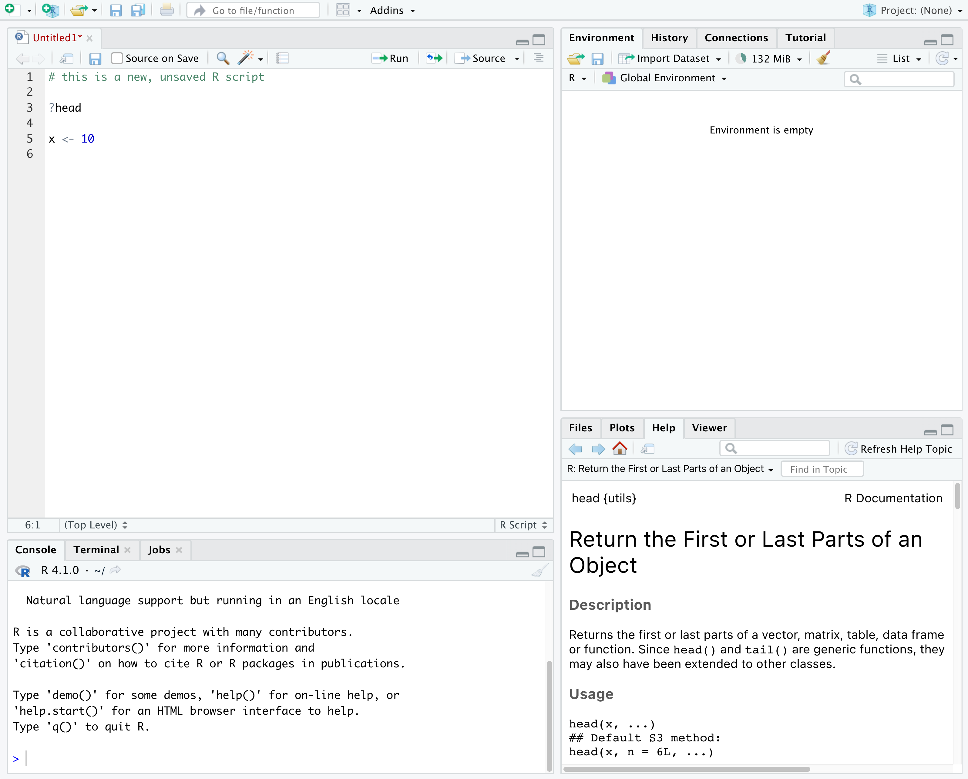 {{alt=‘Screenshot of RStudio showing the 4 “panes”.’}}
In the above screenshot, we can see 4 “panes” in the default layout:
- Top-Left: the Source pane that displays scripts and other files.
- If you only have 3 panes, and the Console pane is in the top left, press Shift+Cmd+N (Mac) or Shift+Ctrl+N (Windows) to open a blank R script, which should make the Source pane appear.
- Top-Right: the Environment/History pane, which shows all the objects in your current R session (Environment) and your command history (History)
- there are some other tabs here, including Connections, Build, Tutorial, and possibly Git
- we won’t cover any of the other tabs, but RStudio has lots of other useful features
- Bottom-Left: the Console pane, where you can interact directly with an R console, which interprets R commands and prints the results
- There are also tabs for Terminal and Jobs
- Bottom-Right: the Files/Plots/Help/Viewer pane to navigate files or view plots and help pages
You can customize the layout of these panes, as well as many settings such as RStudio color scheme, font, and even keyboard shortcuts. You can access these settings by going to the menu bar, then clicking on Tools → Global Options.
RStudio puts most of the things you need to work in R into a single window, and also includes features like keyboard shortcuts, autocompletion of code, and syntax highlighting (different types of code are colored differently, making it easier to navigate your code).
Getting set up in RStudio
It is a good practice to organize your projects into self-contained folders right from the start, so we will start building that habit now. A well-organized project is easier to navigate, more reproducible, and easier to share with others. Your project should start with a top-level folder that contains everything necessary for the project, including data, scripts, and images, all organized into sub-folders.
RStudio provides a “Projects” feature that can make it easier to work on individual projects in R. We will create a project that we will keep everything for this workshop.
- Start RStudio (you should see a view similar to the screenshot above).
- In the top right, you will see a blue 3D cube and the words “Project: (None)”. Click on this icon.
- Click New Project from the dropdown menu.
- Click New Directory, then New Project.
- Type out a name for the project, we recommend
R-Ecology-Workshop. - Put it in a convenient location using the “Create project as a subdirectory of:” section. We recommend your
Desktop. You can always move the project somewhere else later, because it will be self-contained. - Click Create Project and your new project will open.
Next time you open RStudio, you can click that 3D cube icon, and you will see options to open existing projects, like the one you just made.
One of the benefits to using RStudio Projects is that they automatically set the working directory to the top-level folder for the project. The working directory is the folder where R is working, so it views the location of all files (including data and scripts) as being relative to the working directory. You may come across scripts that include something like setwd("/Users/YourUserName/MyCoolProject"), which directly sets a working directory. This is usually much less portable, since that specific directory might not be found on someone else’s computer (they probably don’t have the same username as you). Using RStudio Projects means we don’t have to deal with manually setting the working directory.
There are a few settings we will need to adjust to improve the reproducibility of our work. Go to your menu bar, then click Tools → Global Options to open up the Options window.
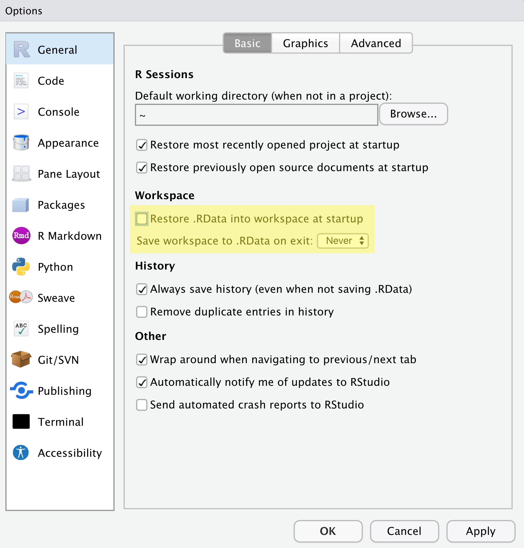
Make sure your settings match those highlighted in yellow. We don’t want RStudio to store the current status of our R session and reload it the next time we start R. This might sound convenient, but for the sake of reproducibility, we want to start with a clean, empty R session every time we work. That means that we have to record everything we do into scripts, save any data we need into files, and store outputs like images as files. We want to get used to everything we generate in a single R session being disposable. We want our scripts to be able to regenerate things we need, other than “raw materials” like data.
Organizing your project directory
Using a consistent folder structure across all your new projects will help keep a growing project organized, and make it easy to find files in the future. This is especially beneficial if you are working on multiple projects, since you will know where to look for particular kinds of files.
We will use a basic structure for this workshop, which is often a good place to start, and can be extended to meet your specific needs. Here is a diagram describing the structure:
R-Ecology-Workshop
│
└── scripts
│
└── data
│    └── cleaned
│    └── raw
│
└─── images
│
└─── documents
Within our project folder (R-Ecology-Workshop), we first have a scripts folder to hold any scripts we write. We also have a data folder containing cleaned and raw subfolders. In general, you want to keep your raw data completely untouched, so once you put data into that folder, you do not modify it. Instead, you read it into R, and if you make any modifications, you write that modified file into the cleaned folder. We also have an images folder for plots we make, and a documents folder for any other documents you might produce.
Let’s start making our new folders. Go to the Files pane (bottom right), and check the current directory, highlighted in yellow below. You should be in the directory for the project you just made, in our case R-Ecology-Workshop. You shouldn’t see any folders in here yet.
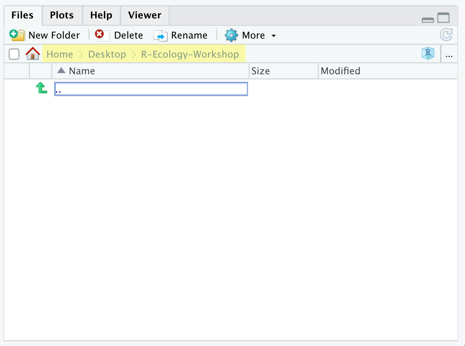
Next, click the New Folder button, and type in scripts to generate your scripts folder. It should appear in the Files list now. Repeat the process to make your data, images, and documents folders. Then, click on the data folder in the Files pane. This will take you into the data folder, which will be empty. Use the New Folder button to create raw and cleaned folders. To return to the R-Ecology-Workshop folder, click on it in the file path, which is highlighted in yellow in the previous image. It’s worth noting that the Files pane helps you create, find, and open files, but moving through your files won’t change where the working directory of your project is.
Working in R and RStudio
The basis of programming is that we write down instructions for the computer to follow, and then we tell the computer to follow those instructions. We write these instructions in the form of code, which is a common language that is understood by the computer and humans (after some practice). We call these instructions commands, and we tell the computer to follow the instructions by running (also called executing) the commands.
Console vs. script
You can run commands directly in the R console, or you can write them into an R script. It may help to think of working in the console vs. working in a script as something like cooking. The console is like making up a new recipe, but not writing anything down. You can carry out a series of steps and produce a nice, tasty dish at the end. However, because you didn’t write anything down, it’s harder to figure out exactly what you did, and in what order.
Writing a script is like taking nice notes while cooking- you can tweak and edit the recipe all you want, you can come back in 6 months and try it again, and you don’t have to try to remember what went well and what didn’t. It’s actually even easier than cooking, since you can hit one button and the computer “cooks” the whole recipe for you!
Console
- The R console is where code is run/executed
- The prompt, which is the
>symbol, is where you can type commands - By pressing Enter, R will execute those commands and print the result.
- You can work here, and your history is saved in the History pane, but you can’t access it in the future
Script
- A script is a record of commands to send to R, preserved in a plain text file with a
.Rextension - You can make a new R script by clicking
File → New File → R Script, clicking the green+button in the top left corner of RStudio, or pressing Shift+Cmd+N (Mac) or Shift+Ctrl+N (Windows). It will be unsaved, and called “Untitled1” - If you type out lines of R code in a script, you can send them to the R console to be evaluated
- Cmd+Enter (Mac) or Ctrl+Enter (Windows) will run the line of code that your cursor is on
- If you highlight multiple lines of code, you can run all of them by pressing Cmd+Enter (Mac) or Ctrl+Enter (Windows)
- By preserving commands in a script, you can edit and rerun them quickly, save them for later, and share them with others
Content from Data visualization with ggplot2
Last updated on 2022-11-29 | Edit this page
Overview
Questions
- How do you make plots using R?
- How do you customize and modify plots?
Objectives
- Produce scatter plots and boxplots using
ggplot2. - Represent data variables with plot components.
- Modify the scales of plot components.
- Iteratively build and modify
ggplot2plots by adding layers. - Change the appearance of existing
ggplot2plots using premade and customized themes. - Describe what faceting is and apply faceting in
ggplot2. - Save plots as image files.
Setup
We are going to be using functions from the ggplot2 package to create visualizations of data. Functions are predefined bits of code that automate more complicated actions. R itself has many built-in functions, but we can access many more by loading other packages of functions and data into R.
If you don’t have a blank, untitled script open yet, go ahead and open one with Shift+Cmd+N (Mac) or Shift+Ctrl+N (Windows). Then save the file to your scripts/ folder, and title it workshop_code.R.
Earlier, you had to install the ggplot2 package by running install.packages("ggplot2"). That installed the package onto your computer so that R can access it. In order to use it in our current session, we have to load the package using the library() function.
Callout
If you do not have ggplot2 installed, you can run install.packages("ggplot2") in the console.
It is a good practice not to put install.packages() into a script. This is because every time you run that whole script, the package will be reinstalled, which is typically unnecessary. You want to install the package to your computer once, and then load it with library() in each script where you need to use it.
R
library(ggplot2)
Later we will learn how to read data from external files into R, but for now we are going to use a clean and ready-to-use dataset that is provided by the ratdat data package. To make our dataset available, we need to load this package too.
R
library(ratdat)
The ratdat package contains data from the Portal Project, which is a long-term dataset from Portal, Arizona, in the Chihuahuan desert.
Let’s take a look at the data briefly. We can use a ? in front of the name of the dataset we’ll be using, which will bring up the help page for the data.
R
?complete_old
Here we can read descriptions of each variable in our data.
We can find out more about the dataset by using the str() function to examine the structure of the data.
R
str(complete_old)
OUTPUT
'data.frame':	16878 obs. of  13 variables:
 $ record_id      : int  1 2 3 4 5 6 7 8 9 10 ...
 $ month          : int  7 7 7 7 7 7 7 7 7 7 ...
 $ day            : int  16 16 16 16 16 16 16 16 16 16 ...
 $ year           : int  1977 1977 1977 1977 1977 1977 1977 1977 1977 1977 ...
 $ plot_id        : int  2 3 2 7 3 1 2 1 1 6 ...
 $ species_id     : chr  "NL" "NL" "DM" "DM" ...
 $ sex            : chr  "M" "M" "F" "M" ...
 $ hindfoot_length: int  32 33 37 36 35 14 NA 37 34 20 ...
 $ weight         : int  NA NA NA NA NA NA NA NA NA NA ...
 $ genus          : chr  "Neotoma" "Neotoma" "Dipodomys" "Dipodomys" ...
 $ species        : chr  "albigula" "albigula" "merriami" "merriami" ...
 $ taxa           : chr  "Rodent" "Rodent" "Rodent" "Rodent" ...
 $ plot_type      : chr  "Control" "Long-term Krat Exclosure" "Control" "Rodent Exclosure" ...
str() will tell us how many observations/rows (obs) and variables/columns we have, as well as some information about each of the variables. We see the name of a variable (such as year), followed by the kind of variable (int for integer, chr for character), and the first 10 entries in that variable. We will talk more about different data types and structures later on.
Plotting with ggplot2
ggplot2 is a powerful package that allows you to create complex plots from tabular data (data in a table format with rows and columns). The gg in ggplot2 stands for “grammar of graphics”, and the package uses consistent vocabulary to create plots of widely varying types. Therefore, we only need small changes to our code if the underlying data changes or we decide to make a box plot instead of a scatter plot. This approach helps you create publication-quality plots with minimal adjusting and tweaking.
ggplot2 is part of the tidyverse series of packages, which tend to like data in the “long” or “tidy” format, which means each column represents a single variable, and each row represents a single observation. Well-structured data will save you lots of time making figures with ggplot2. For now, we will use data that are already in this format. We start learning R by using ggplot2 because it relies on concepts that we will need when we talk about data transformation in the next lessons.
ggplot plots are built step by step by adding new layers, which allows for extensive flexibility and customization of plots.
To build a plot, we will use a basic template that can be used for different types of plots:
R
ggplot(data = <DATA>, mapping = aes(<MAPPINGS>)) + <GEOM_FUNCTION>()We use the ggplot() function to create a plot. In order to tell it what data to use, we need to specify the data argument. An argument is an input that a function takes, and you set arguments using the = sign.
R
ggplot(data = complete_old)

We get a blank plot because we haven’t told ggplot() which variables we want to correspond to parts of the plot. We can specify the “mapping” of variables to plot elements, such as x/y coordinates, size, or shape, by using the aes() function. We’ll also add a comment, which is any line starting with a #. It’s a good idea to use comments to organize your code or clarify what you are doing.
R
# adding a mapping to x and y axes
ggplot(data = complete_old, mapping = aes(x = weight, y = hindfoot_length))
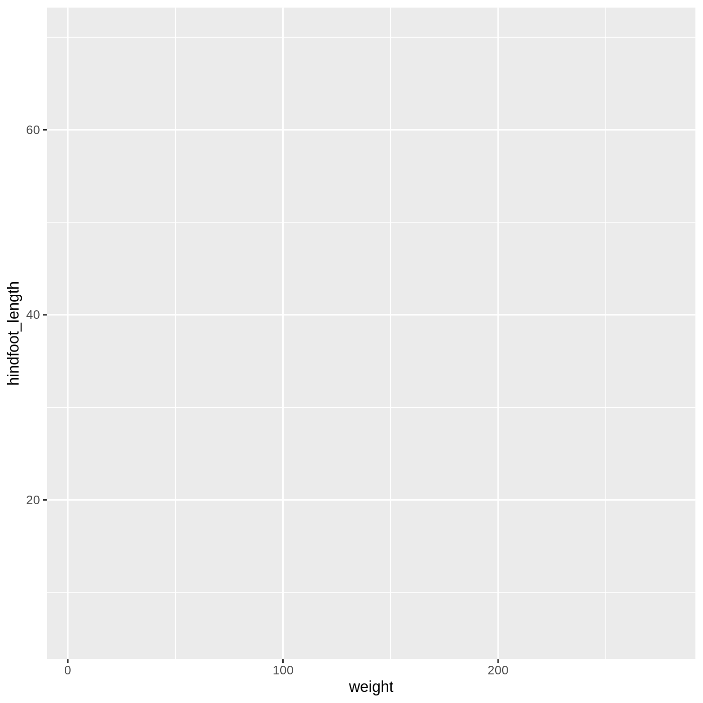
Now we’ve got a plot with x and y axes corresponding to variables from complete_old. However, we haven’t specified how we want the data to be displayed. We do this using geom_ functions, which specify the type of geometry we want, such as points, lines, or bars. We can add a geom_point() layer to our plot by using the + sign. We indent onto a new line to make it easier to read, and we have to end the first line with the + sign.
R
ggplot(data = complete_old, mapping = aes(x = weight, y = hindfoot_length)) +
  geom_point()
WARNING
Warning: Removed 3081 rows containing missing values (geom_point).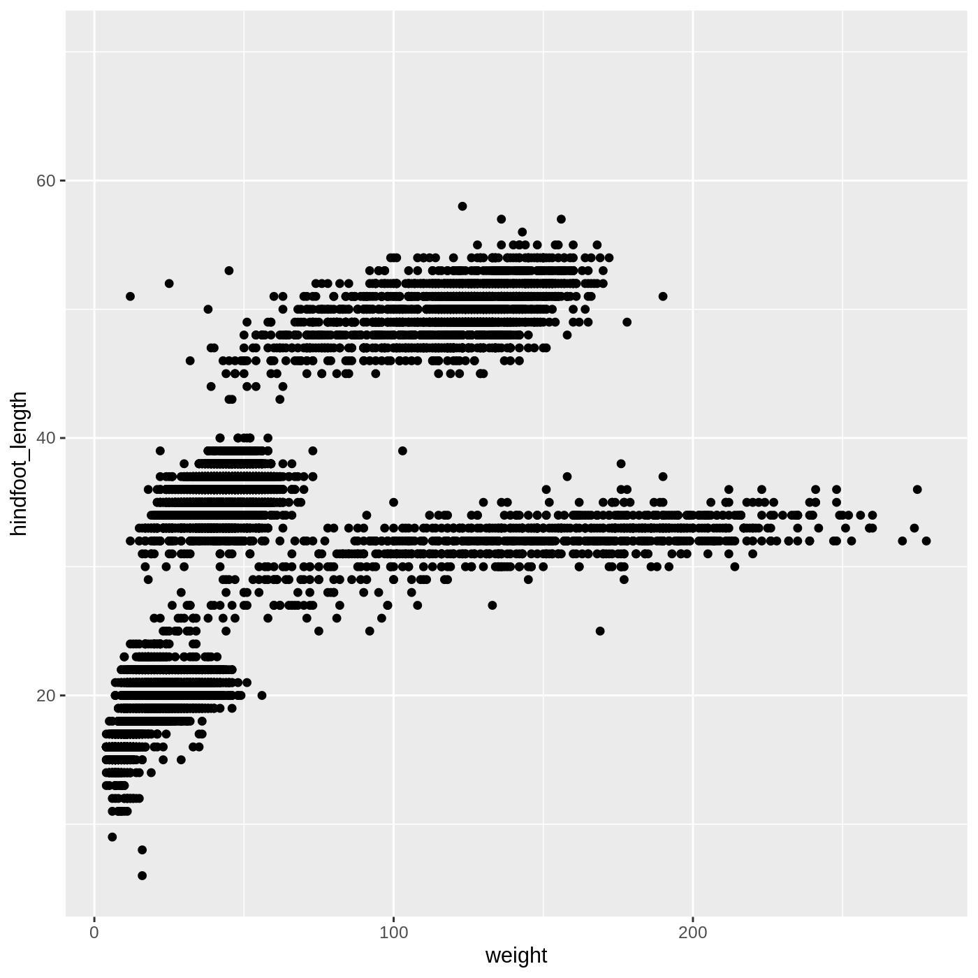
You may notice a warning that missing values were removed. If a variable necessary to make the plot is missing from a given row of data (in this case, hindfoot_length or weight), it can’t be plotted. ggplot2 just uses a warning message to let us know that some rows couldn’t be plotted.
Callout
Warning messages are one of a few ways R will communicate with you. Warnings can be thought of as a “heads up”. Nothing necessarily went wrong, but the author of that function wanted to draw your attention to something. In the above case, it’s worth knowing that some of the rows of your data were not plotted because they had missing data.
A more serious type of message is an error. Here’s an example:
R
ggplot(data = complete_old, mapping = aes(x = weight, y = hindfoot_length)) +
  geom_poit()
ERROR
Error in geom_poit(): could not find function "geom_poit"As you can see, we only get the error message, with no plot, because something has actually gone wrong. This particular error message is fairly common, and it happened because we misspelled point as poit. Because there is no function named geom_poit(), R tells us it can’t find a function with that name.
Changing aesthetics
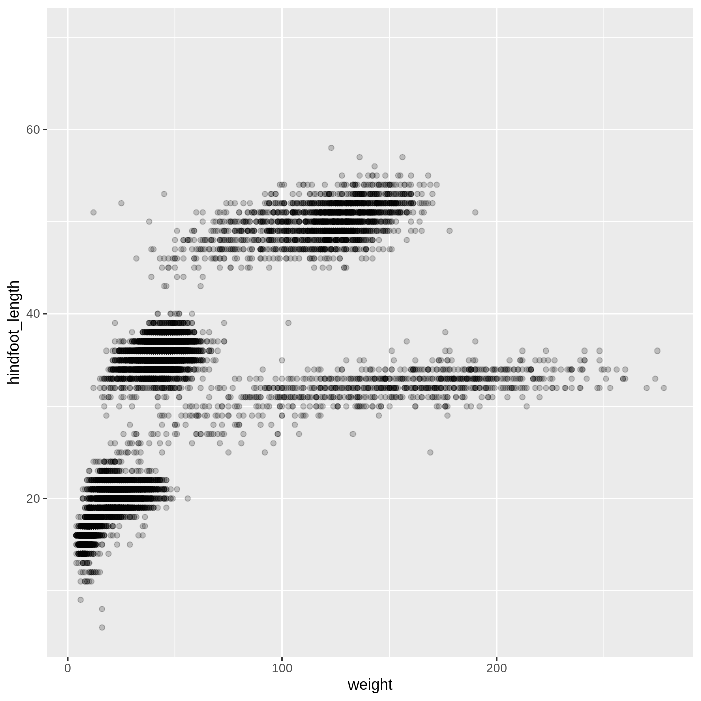
Building ggplot plots is often an iterative process, so we’ll continue developing the scatter plot we just made. You may have noticed that parts of our scatter plot have many overlapping points, making it difficult to see all the data. We can adjust the transparency of the points using the alpha argument, which takes a value between 0 and 1:
R
ggplot(data = complete_old, mapping = aes(x = weight, y = hindfoot_length)) +
  geom_point(alpha = 0.2)
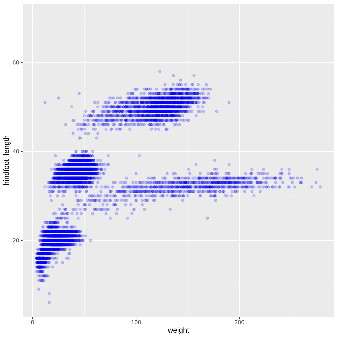
We can also change the color of the points:
R
ggplot(data = complete_old, mapping = aes(x = weight, y = hindfoot_length)) +
  geom_point(alpha = 0.2, color = "blue")
Callout
Two common issues you might run into when working in R are forgetting a closing bracket or a closing quote. Let’s take a look at what each one does.
Try running the following code:
R
ggplot(data = complete_old, mapping = aes(x = weight, y = hindfoot_length)) +
  geom_point(color = "blue", alpha = 0.2
You will see a + appear in your console. This is R telling you that it expects more input in order to finish running the code. It is missing a closing bracket to end the geom_point function call. You can hit Esc in the console to reset it.
Something similar will happen if you run the following code:
R
ggplot(data = complete_old, mapping = aes(x = weight, y = hindfoot_length)) +
  geom_point(color = "blue, alpha = 0.2)
A missing quote at the end of blue means that the rest of the code is treated as part of the quote, which is a bit easier to see since RStudio displays character strings in a different color.
You will get a different error message if you run the following code:
R
ggplot(data = complete_old, mapping = aes(x = weight, y = hindfoot_length)) +
  geom_point(color = "blue", alpha = 0.2))
This time we have an extra closing ), which R doesn’t know what to do with. It tells you there is an unexpected ), but it doesn’t pinpoint exactly where. With enough time working in R, you will get better at spotting mismatched brackets.
Adding another variable
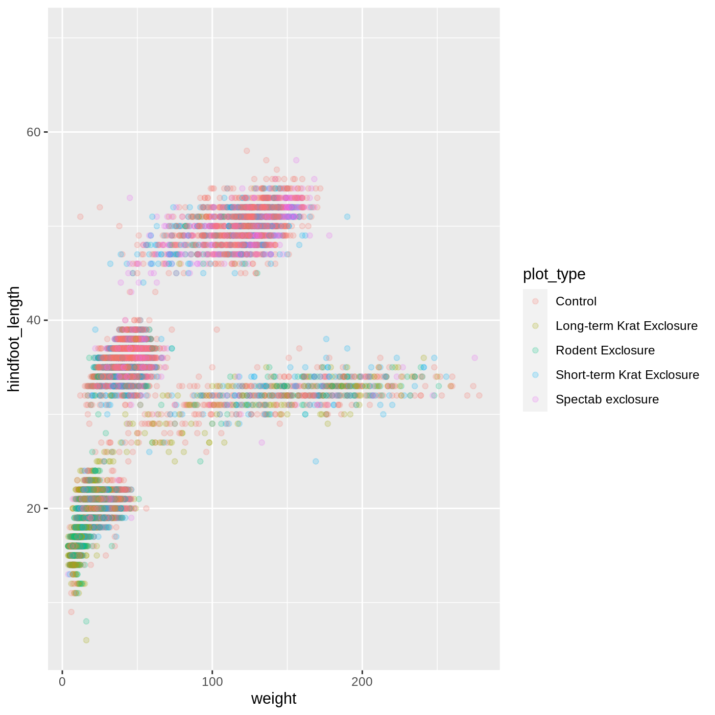
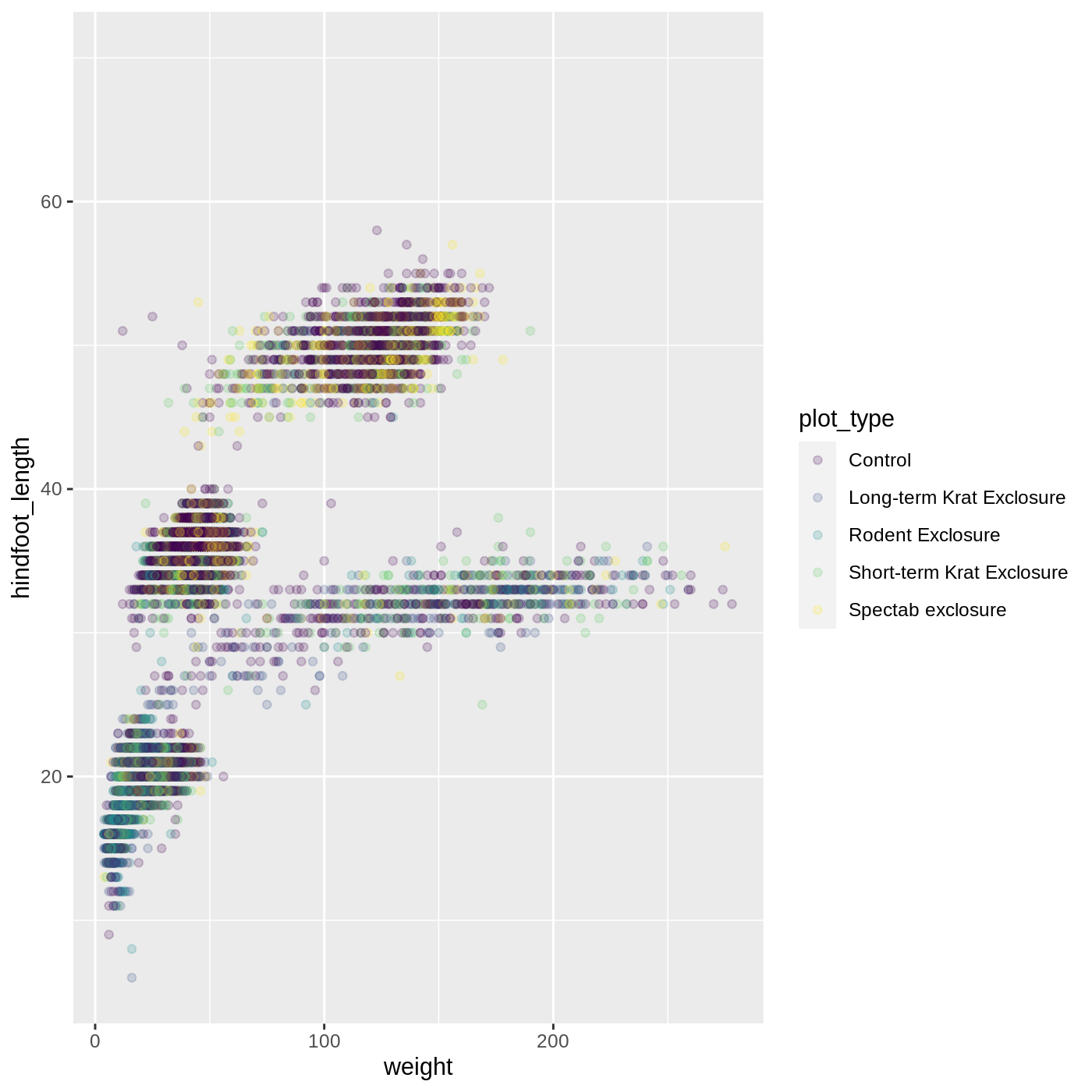
Let’s try coloring our points according to the plot type. Since we’re now mapping a variable (plot_type) to a component of the plot (color), we need to put the argument inside aes():
R
ggplot(data = complete_old, mapping = aes(x = weight, y = hindfoot_length, color = plot_type)) +
  geom_point(alpha = 0.2)
R
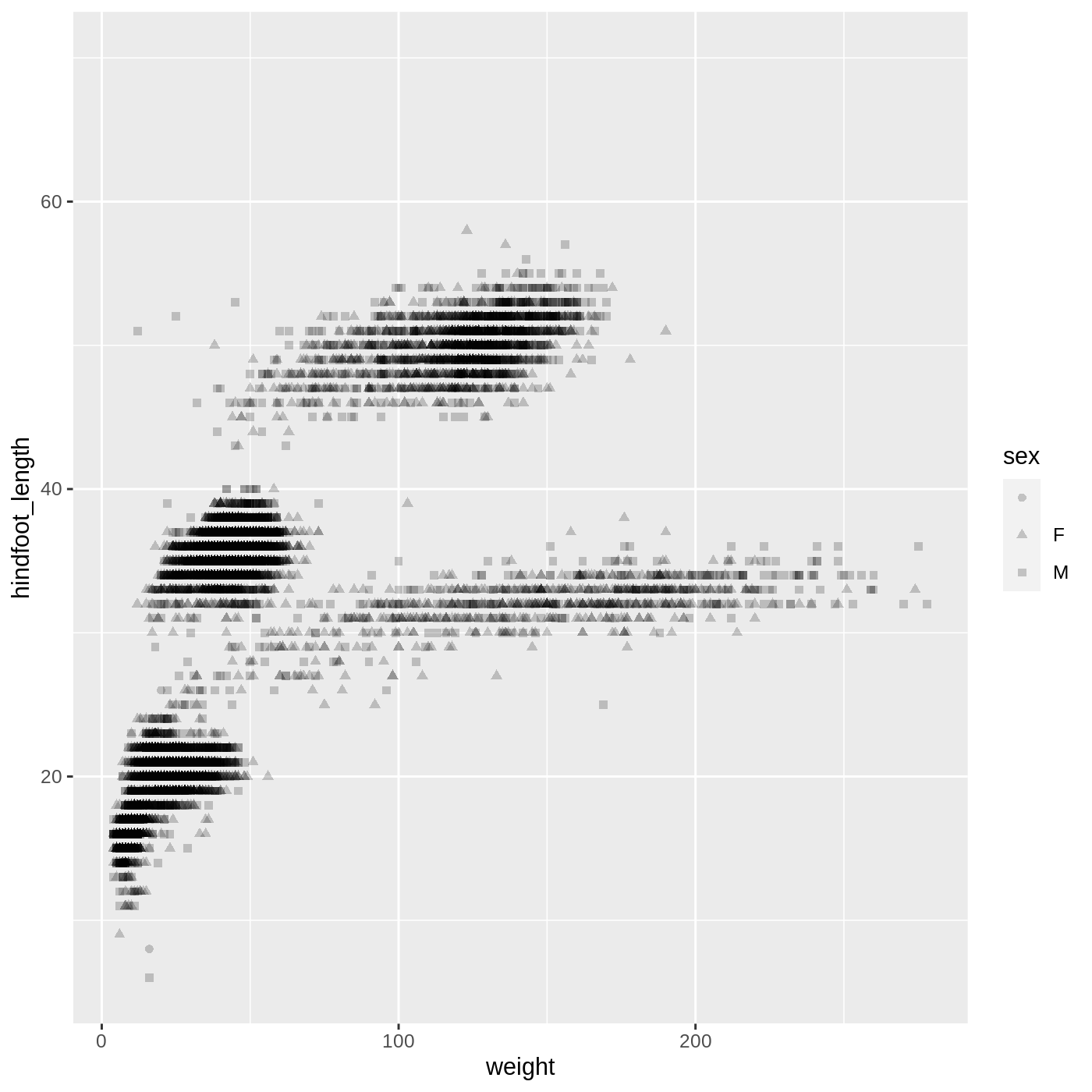
ggplot(data = complete_old,
       mapping = aes(x = weight, y = hindfoot_length, shape = sex)) +
  geom_point(alpha = 0.2)
R
ggplot(data = complete_old,
       mapping = aes(x = weight, y = hindfoot_length, color = year)) +
  geom_point(alpha = 0.2)
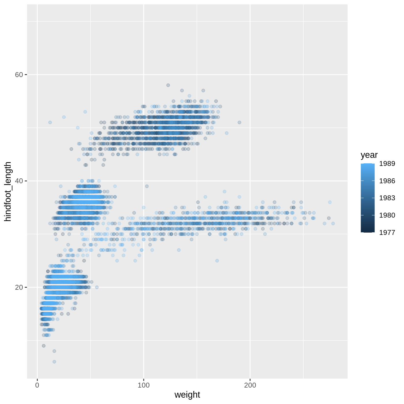
- For Part 2, the color scale is different compared to using
color = plot_typebecauseplot_typeandyearare different variable types.plot_typeis a categorical variable, soggplot2defaults to use a discrete color scale, whereasyearis a numeric variable, soggplot2uses a continuous color scale.
Changing scales
The default discrete color scale isn’t always ideal: it isn’t friendly to viewers with colorblindness and it doesn’t translate well to grayscale. However, ggplot2 comes with quite a few other color scales, including the fantastic viridis scales, which are designed to be colorblind and grayscale friendly. We can change scales by adding scale_ functions to our plots:
R
ggplot(data = complete_old, mapping = aes(x = weight, y = hindfoot_length, color = plot_type)) +
  geom_point(alpha = 0.2) +
  scale_color_viridis_d()
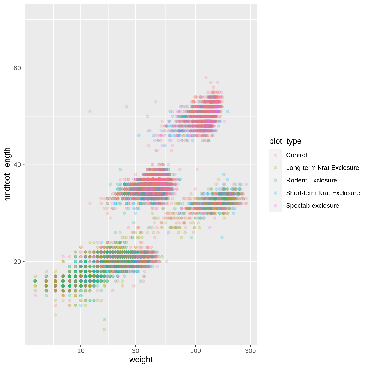
Scales don’t just apply to colors- any plot component that you put inside aes() can be modified with scale_ functions. Just as we modified the scale used to map plot_type to color, we can modify the way that weight is mapped to the x axis by using the scale_x_log10() function:
R
ggplot(data = complete_old, mapping = aes(x = weight, y = hindfoot_length, color = plot_type)) +
  geom_point(alpha = 0.2) +
  scale_x_log10()
One nice thing about ggplot and the tidyverse in general is that groups of functions that do similar things are given similar names. Any function that modifies a ggplot scale starts with scale_, making it easier to search for the right function.
Boxplot
Let’s try making a different type of plot altogether. We’ll start off with our same basic building blocks using ggplot() and aes().
R
ggplot(data = complete_old, mapping = aes(x = plot_type, y = hindfoot_length))
This time, let’s try making a boxplot, which will have plot_type on the x axis and hindfoot_length on the y axis. We can do this by adding geom_boxplot() to our ggplot():
R
ggplot(data = complete_old, mapping = aes(x = plot_type, y = hindfoot_length)) +
  geom_boxplot()
WARNING
Warning: Removed 2733 rows containing non-finite values (stat_boxplot).
Just as we colored the points before, we can color our boxplot by plot_type as well:
R
ggplot(data = complete_old, mapping = aes(x = plot_type, y = hindfoot_length, color = plot_type)) +
  geom_boxplot()
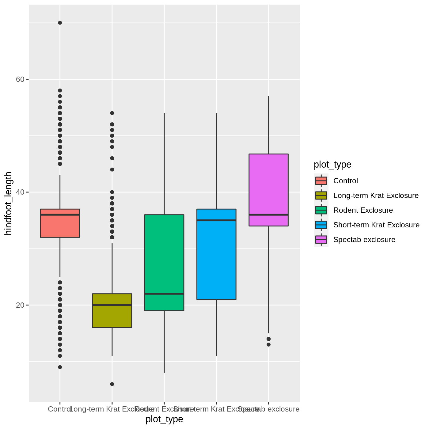
It looks like color has only affected the outlines of the boxplot, not the rectangular portions. This is because the color only impacts 1-dimensional parts of a ggplot: points and lines. To change the color of 2-dimensional parts of a plot, we use fill:
R
ggplot(data = complete_old, mapping = aes(x = plot_type, y = hindfoot_length, fill = plot_type)) +
  geom_boxplot()
Callout
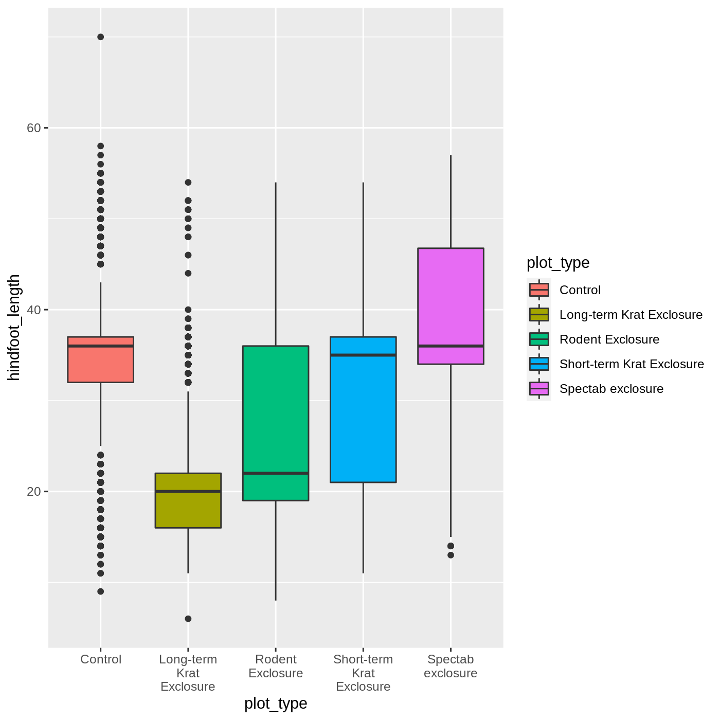
One thing you may notice is that the axis labels are overlapping each other, depending on how wide your plot viewer is. One way to help make them more legible is to wrap the text. We can do that by modifying the labels for the x axis scale.
We use the scale_x_discrete() function because we have a discrete axis, and we modify the labels argument. The function label_wrap_gen() will wrap the text of the labels to make them more legible.
R
ggplot(data = complete_old, mapping = aes(x = plot_type, y = hindfoot_length, fill = plot_type)) +
  geom_boxplot() +
  scale_x_discrete(labels = label_wrap_gen(width = 10))
Adding geoms
One of the most powerful aspects of ggplot is the way we can add components to a plot in successive layers. While boxplots can be very useful for summarizing data, it is often helpful to show the raw data as well. With ggplot, we can easily add another geom_ to our plot to show the raw data.
Let’s add geom_point() to visualize the raw data. We will modify the alpha argument to help with overplotting.
R
ggplot(data = complete_old, mapping = aes(x = plot_type, y = hindfoot_length)) +
  geom_boxplot() +
  geom_point(alpha = 0.2)
Uh oh… all our points for a given x axis category fall exactly on a line, which isn’t very useful. We can shift to using geom_jitter(), which will add points with a bit of random noise added to the positions to prevent this from happening.
R
ggplot(data = complete_old, mapping = aes(x = plot_type, y = hindfoot_length)) +
  geom_boxplot() +
  geom_jitter(alpha = 0.2)
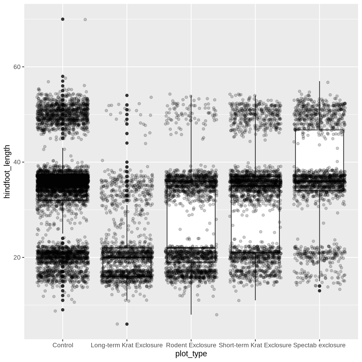
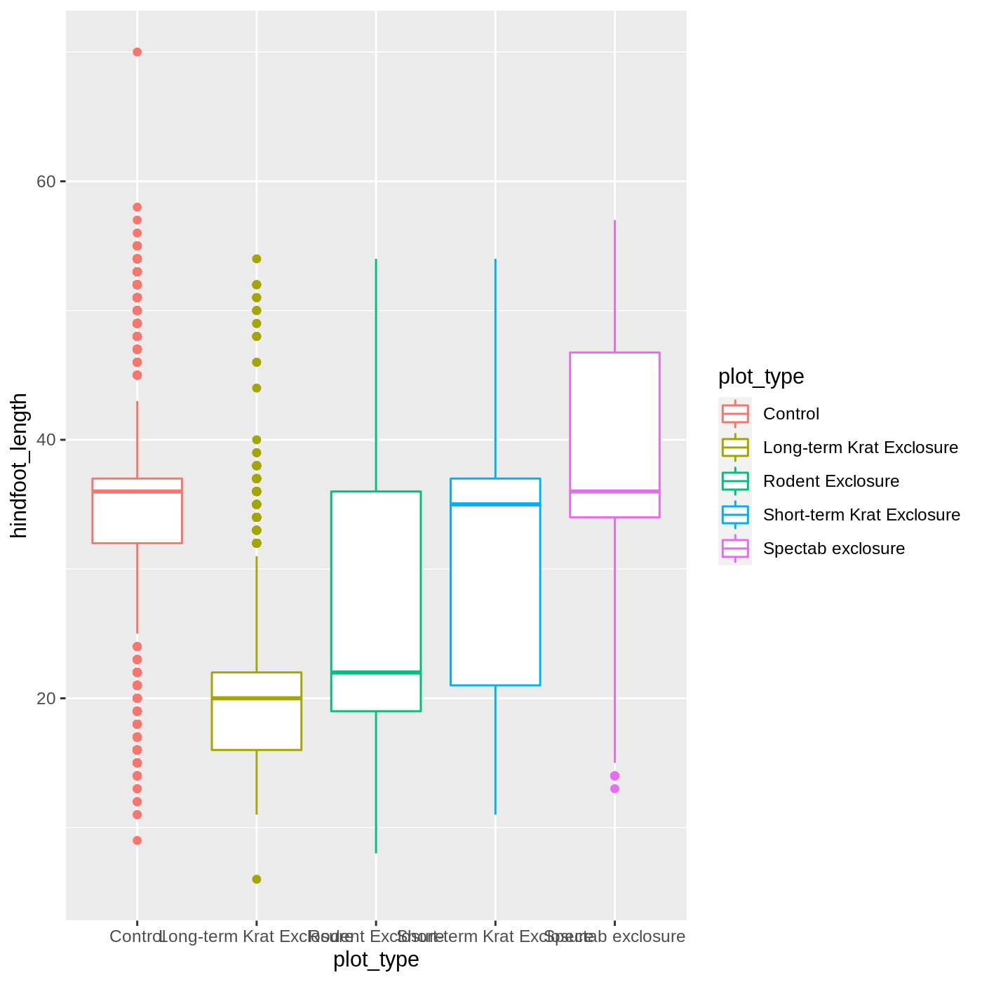
You may have noticed that some of our data points are now appearing on our plot twice: the outliers are plotted as black points from geom_boxplot(), but they are also plotted with geom_jitter(). Since we don’t want to represent these data multiple times in the same form (points), we can stop geom_boxplot() from plotting them. We do this by setting the outlier.shape argument to NA, which means the outliers don’t have a shape to be plotted.
R
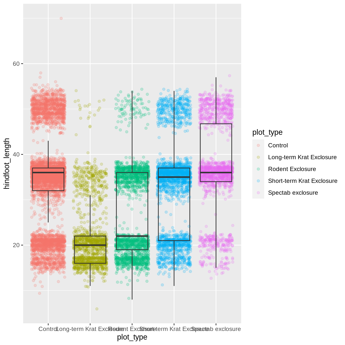
ggplot(data = complete_old, mapping = aes(x = plot_type, y = hindfoot_length)) +
  geom_boxplot(outlier.shape = NA) +
  geom_jitter(alpha = 0.2)
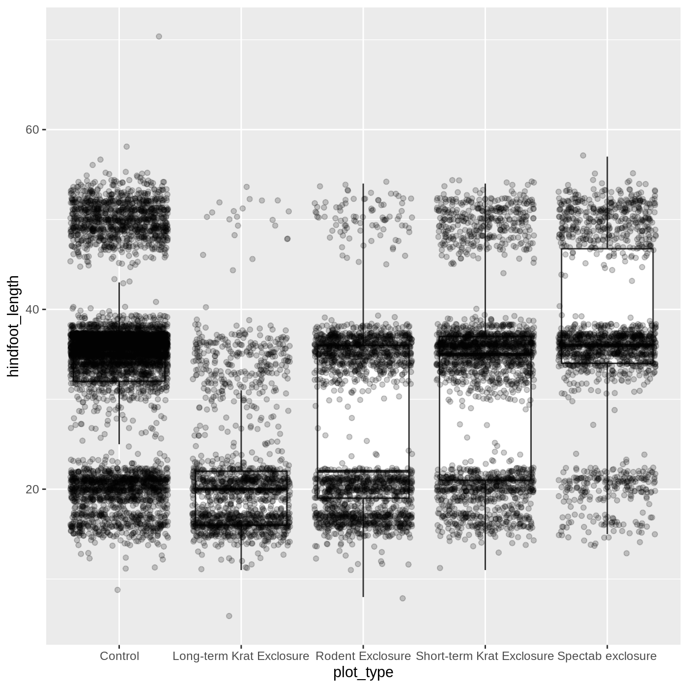
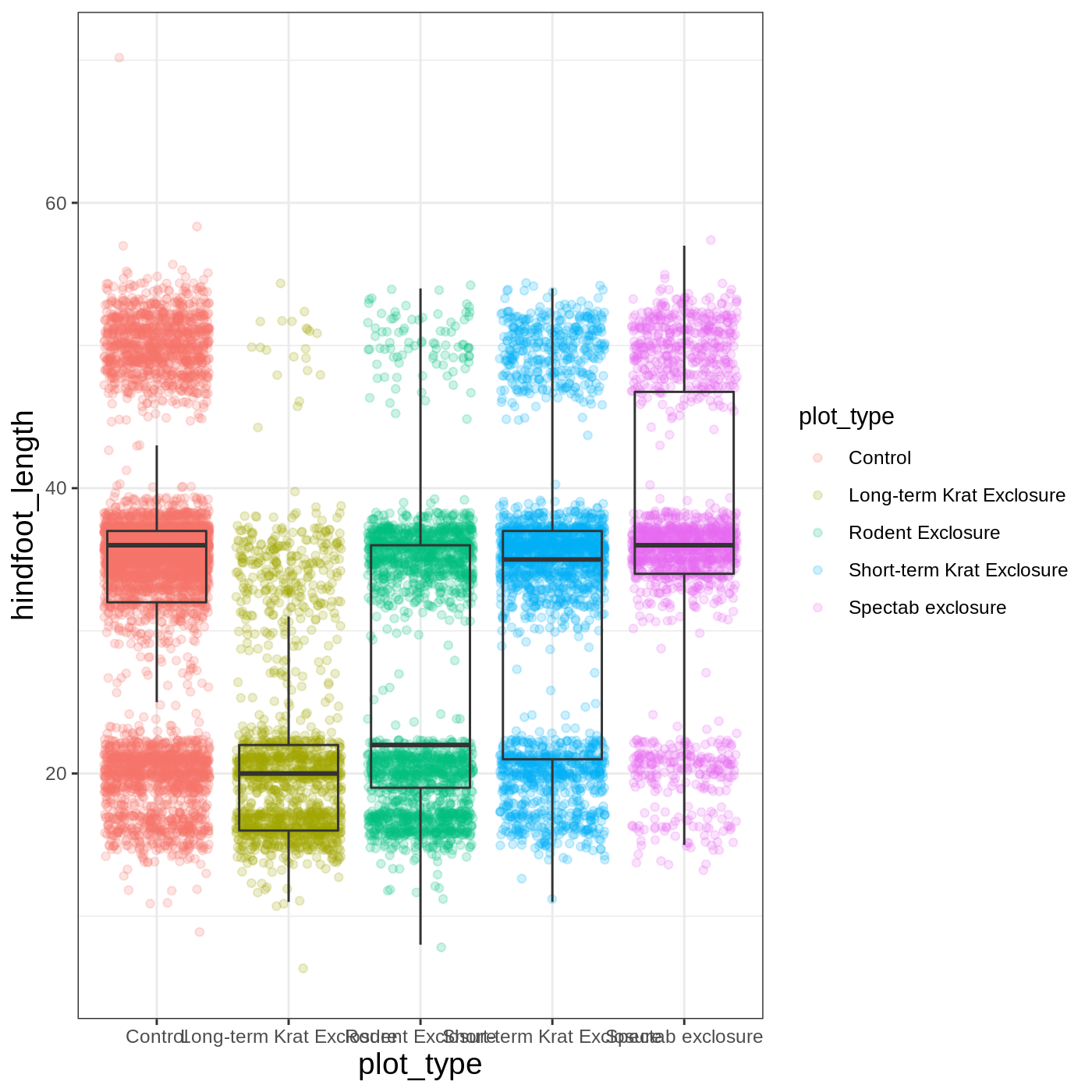
Just as before, we can map plot_type to color by putting it inside aes().
R
ggplot(data = complete_old, mapping = aes(x = plot_type, y = hindfoot_length, color = plot_type)) +
  geom_boxplot(outlier.shape = NA) +
  geom_jitter(alpha = 0.2)

Notice that both the color of the points and the color of the boxplot lines changed. Any time we specify an aes() mapping inside our initial ggplot() function, that mapping will apply to all our geoms.
If we want to limit the mapping to a single geom, we can put the mapping into the specific geom_ function, like this:
R
ggplot(data = complete_old, mapping = aes(x = plot_type, y = hindfoot_length)) +
  geom_boxplot(outlier.shape = NA) +
  geom_jitter(aes(color = plot_type), alpha = 0.2)
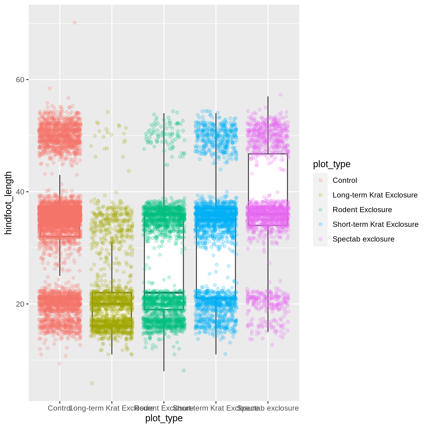
Now our points are colored according to plot_type, but the boxplots are all the same color. One thing you might notice is that even with alpha = 0.2, the points obscure parts of the boxplot. This is because the geom_point() layer comes after the geom_boxplot() layer, which means the points are plotted on top of the boxes. To put the boxplots on top, we switch the order of the layers:
R
ggplot(data = complete_old, mapping = aes(x = plot_type, y = hindfoot_length)) +
  geom_jitter(aes(color = plot_type), alpha = 0.2) +
  geom_boxplot(outlier.shape = NA)
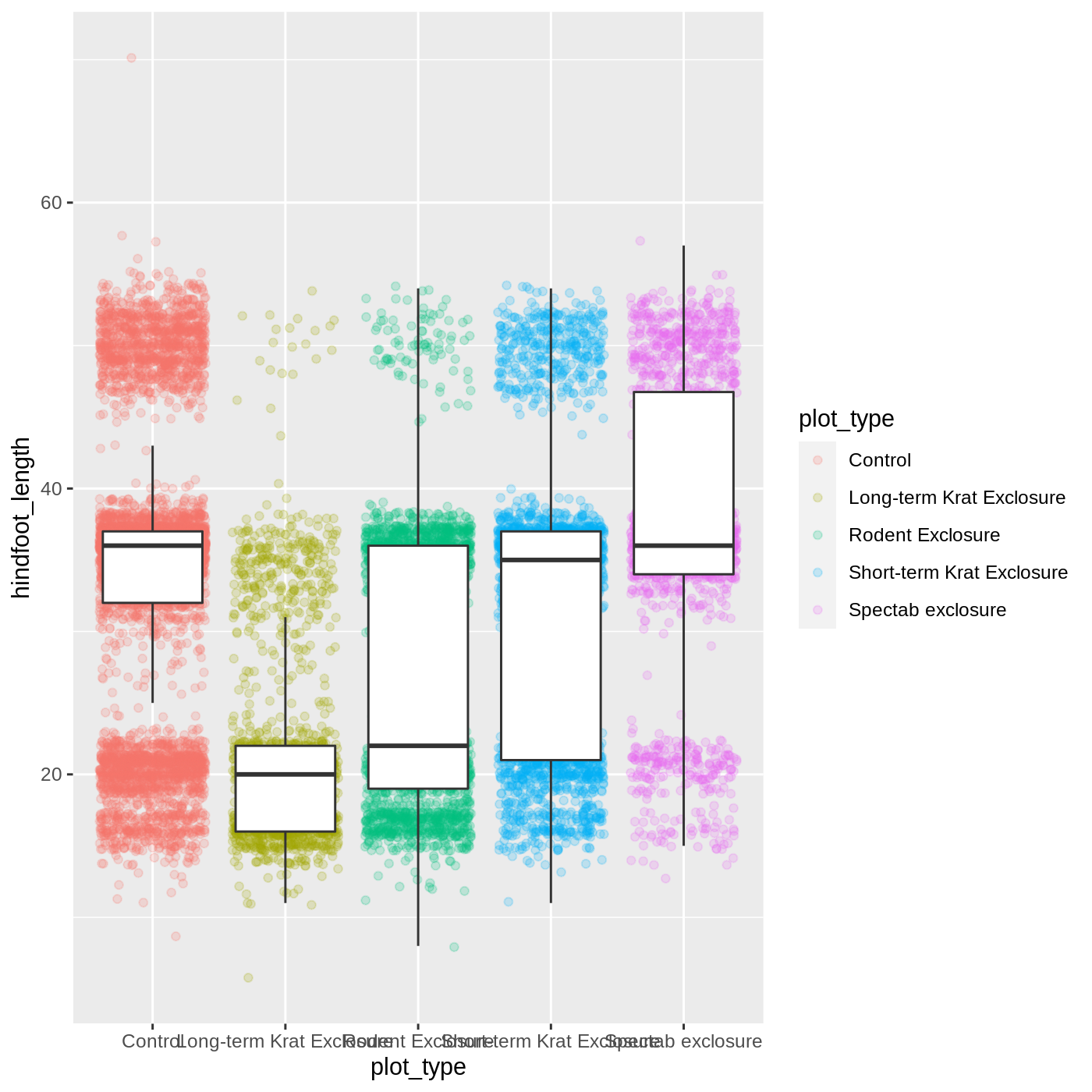
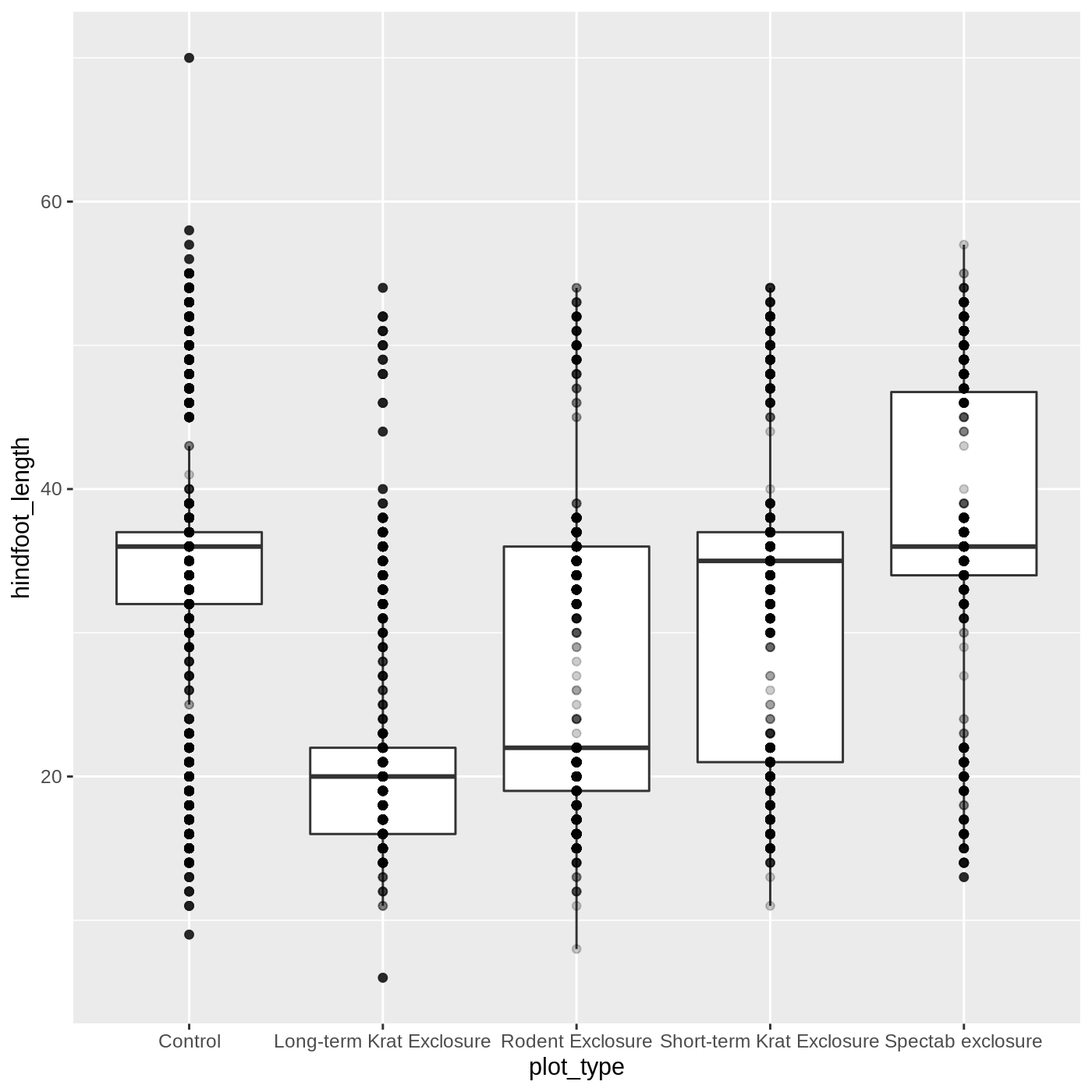
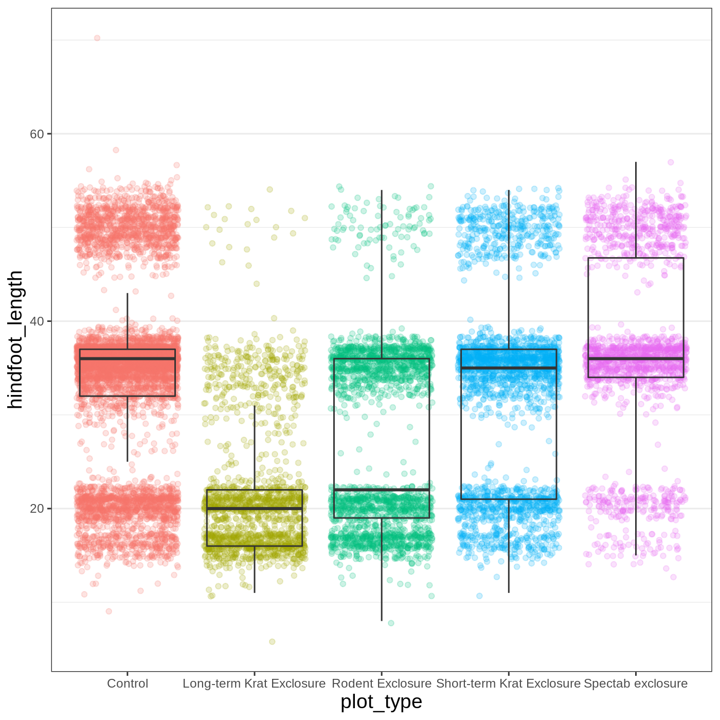
Now we have the opposite problem! The white fill of the boxplots completely obscures some of the points. To address this problem, we can remove the fill from the boxplots altogether, leaving only the black lines. To do this, we set fill to NA:
R
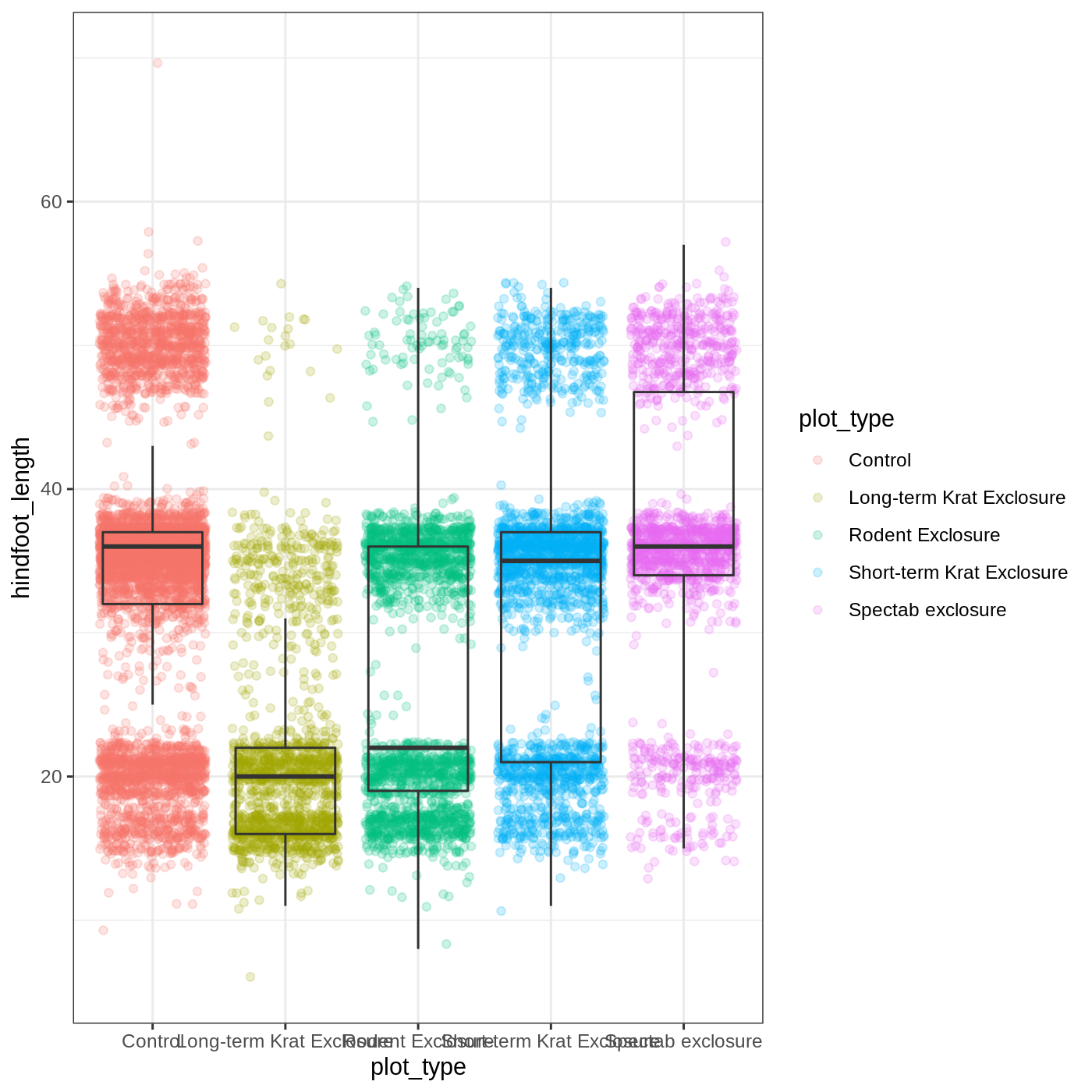
ggplot(data = complete_old, mapping = aes(x = plot_type, y = hindfoot_length)) +
  geom_jitter(aes(color = plot_type), alpha = 0.2) +
  geom_boxplot(outlier.shape = NA, fill = NA)
Now we can see all the raw data and our boxplots on top.
Challenge 2: Change geoms
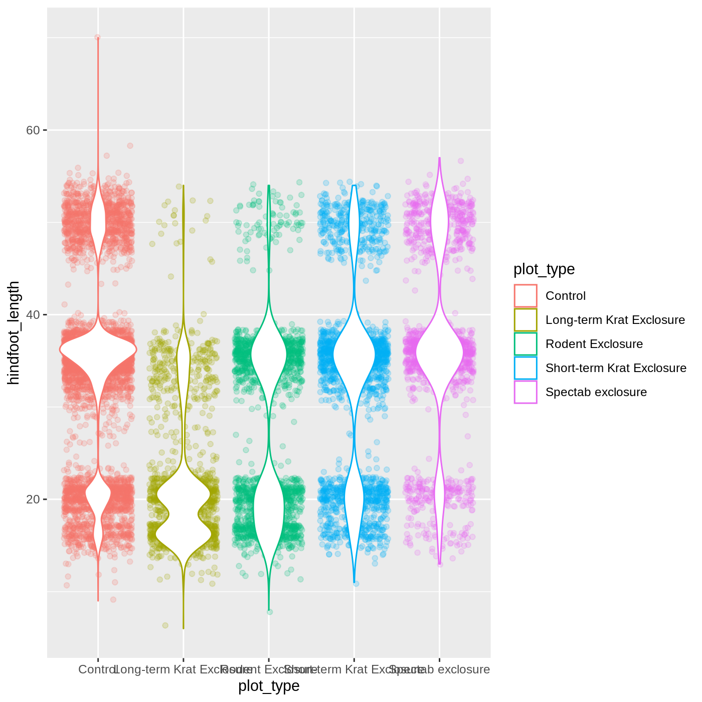
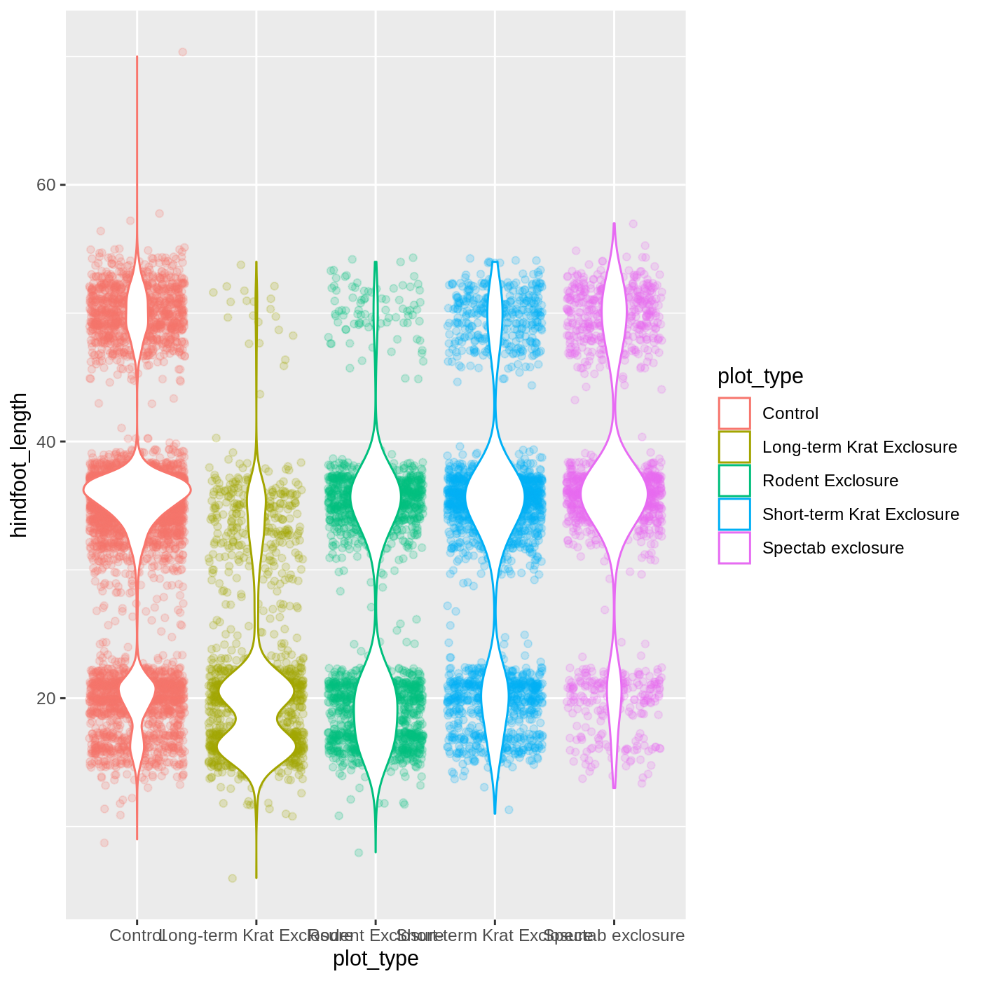
Violin plots are similar to boxplots- try making one using plot_type and hindfoot_length as the x and y variables. Remember that all geom functions start with geom_, followed by the type of geom.
This might also be a place to test your search engine skills. It is often useful to search for R package_name stuff you want to search. So for this example we might search for R ggplot2 violin plot.
R
ggplot(data = complete_old,
       mapping = aes(x = plot_type,
                     y = hindfoot_length,
                     color = plot_type)) +
  geom_jitter(alpha = 0.2) +
  geom_violin(fill = "white")
R
ggplot(data = complete_old,
       mapping = aes(x = plot_type,
                     y = hindfoot_length,
                     color = plot_type)) +
  geom_jitter(alpha = 0.2) +
  geom_violin(fill = "white")
Changing themes
So far we’ve been changing the appearance of parts of our plot related to our data and the geom_ functions, but we can also change many of the non-data components of our plot.
At this point, we are pretty happy with the basic layout of our plot, so we can assign it to a plot to a named object. We do this using the assignment arrow <-. We will create an object called myplot. If you run the name of the ggplot2 object, it will show the plot, just like if you ran the code itself.
R
myplot <- ggplot(data = complete_old, mapping = aes(x = plot_type, y = hindfoot_length)) +
  geom_jitter(aes(color = plot_type), alpha = 0.2) +
  geom_boxplot(outlier.shape = NA, fill = NA)

myplot
WARNING
Warning: Removed 2733 rows containing non-finite values (stat_boxplot).WARNING
Warning: Removed 2733 rows containing missing values (geom_point).
This process of assigning something to an object is not specific to ggplot2, but rather a general feature of R. We will be using it a lot in the rest of this lesson. We can now work with the myplot object as if it was a block of ggplot2 code, which means we can use + to add new components to it.
We can change the overall appearance using theme_ functions. Let’s try a black-and-white theme by adding theme_bw() to our plot:
R
myplot + theme_bw()
As you can see, a number of parts of the plot have changed. theme_ functions usually control many aspects of a plot’s appearance all at once, for the sake of convenience. To individually change parts of a plot, we can use the theme() function, which can take many different arguments to change things about the text, grid lines, background color, and more. Let’s try changing the size of the text on our axis titles. We can do this by specifying that the axis.title should be an element_text() with size set to 14.
R
myplot +
  theme_bw() +
  theme(axis.title = element_text(size = 14))
Another change we might want to make is to remove the vertical grid lines. Since our x axis is categorical, those grid lines aren’t useful. To do this, inside theme(), we will change the panel.grid.major.x to an element_blank().
R
myplot +
  theme_bw() +
  theme(axis.title = element_text(size = 14),
        panel.grid.major.x = element_blank())
Another useful change might be to remove the color legend, since that information is already on our x axis. For this one, we will set legend.position to “none”.
R
myplot +
  theme_bw() +
  theme(axis.title = element_text(size = 14),
        panel.grid.major.x = element_blank(),
        legend.position = "none")
Callout
Because there are so many possible arguments to the theme() function, it can sometimes be hard to find the right one. Here are some tips for figuring out how to modify a plot element:
- type out
theme(), put your cursor between the parentheses, and hit Tab to bring up a list of arguments- you can scroll through the arguments, or start typing, which will shorten the list of potential matches
- like many things in the
tidyverse, similar argument start with similar names- there are
axis,legend,panel,plot, andstriparguments
- there are
- arguments have hierarchy
-
textcontrols all text in the whole plot -
axis.titlecontrols the text for the axis titles -
axis.title.xcontrols the text for the x axis title
-
Changing labels
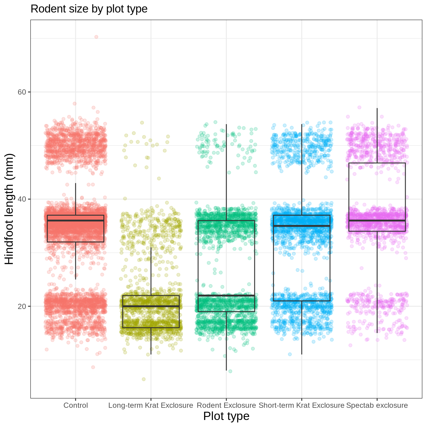
Our plot is really shaping up now. However, we probably want to make our axis titles nicer, and perhaps add a main title to the plot. We can do this using the labs() function:
R
myplot +
  theme_bw() +
  theme(axis.title = element_text(size = 14),
        legend.position = "none") +
  labs(title = "Rodent size by plot type",
       x = "Plot type",
       y = "Hindfoot length (mm)")
We removed our legend from this plot, but you can also change the titles of various legends using labs(). For example, labs(color = "Plot type") would change the title of a color scale legend to “Plot type”.
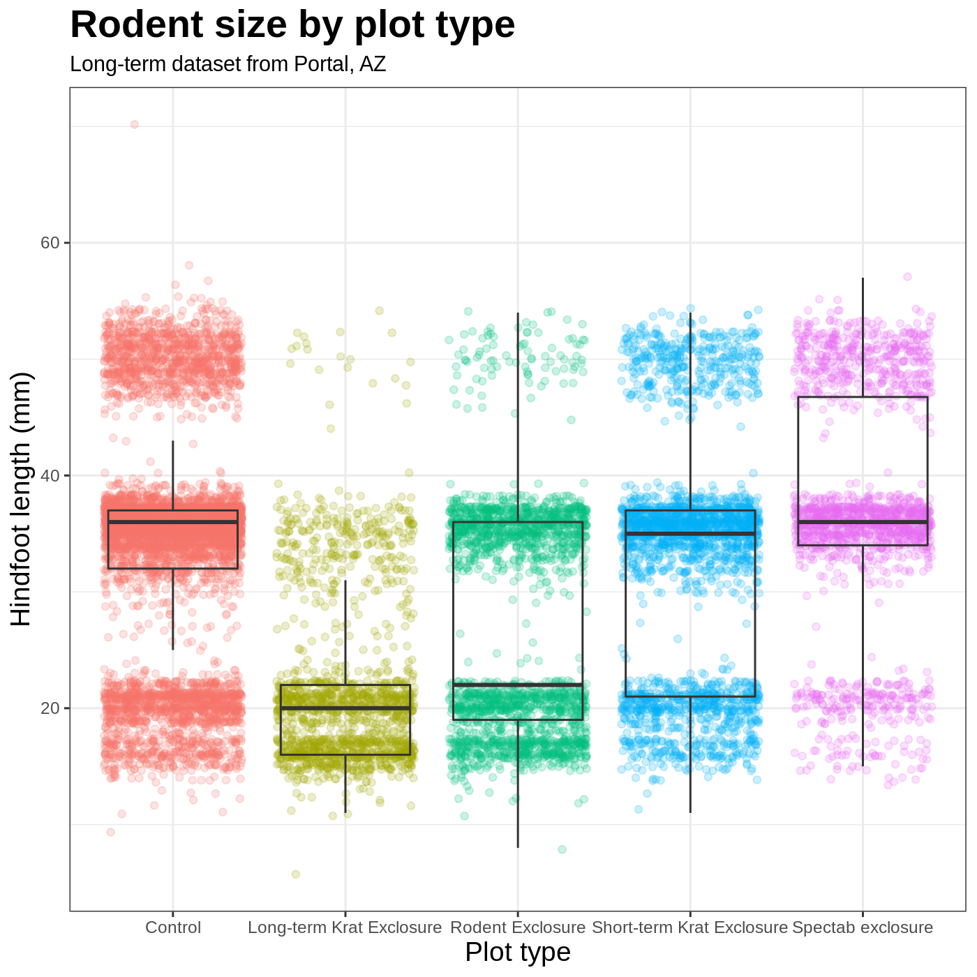
R
myplot +
  theme_bw() +
  theme(axis.title = element_text(size = 14), legend.position = "none",
        plot.title = element_text(face = "bold", size = 20)) +
  labs(title = "Rodent size by plot type",
       subtitle = "Long-term dataset from Portal, AZ",
       x = "Plot type",
       y = "Hindfoot length (mm)")
Faceting
One of the most powerful features of ggplot is the ability to quickly split a plot into multiple smaller plots based on a categorical variable, which is called faceting.
So far we’ve mapped variables to the x axis, the y axis, and color, but trying to add a 4th variable becomes difficult. Changing the shape of a point might work, but only for very few categories, and even then, it can be hard to tell the differences between the shapes of small points.
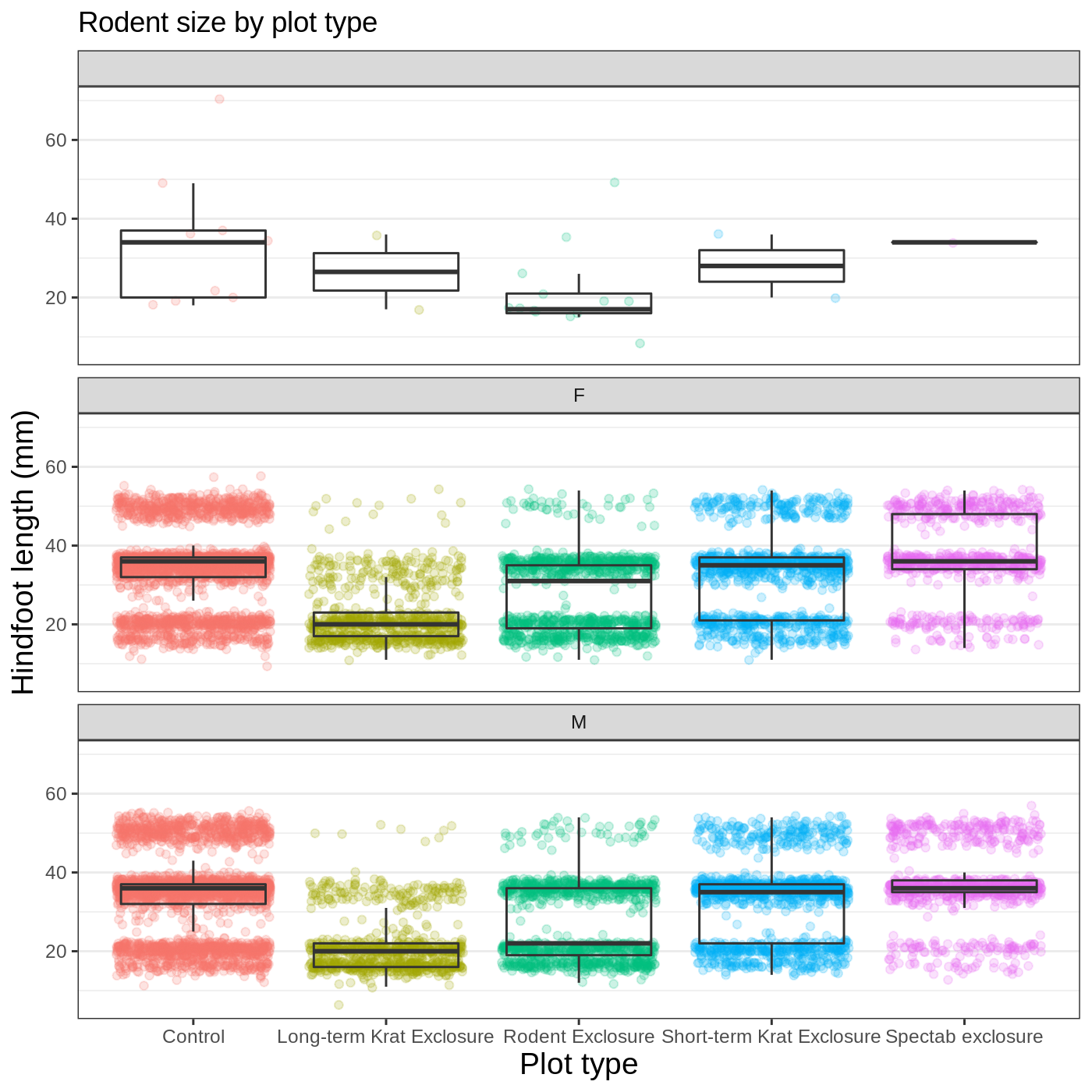
Instead of cramming one more variable into a single plot, we will use the facet_wrap() function to generate a series of smaller plots, split out by sex. We also use ncol to specify that we want them arranged in a single column:
R
myplot +
  theme_bw() +
  theme(axis.title = element_text(size = 14),
        legend.position = "none",
        panel.grid.major.x = element_blank()) +
  labs(title = "Rodent size by plot type",
       x = "Plot type",
       y = "Hindfoot length (mm)",
       color = "Plot type") +
  facet_wrap(vars(sex), ncol = 1)
Callout
Faceting comes in handy in many scenarios. It can be useful when:
- a categorical variable has too many levels to differentiate by color (such as a dataset with 20 countries)
- your data overlap heavily, obscuring categories
- you want to show more than 3 variables at once
- you want to see each category in isolation while allowing for general comparisons between categories
Exporting plots
Once we are happy with our final plot, we can assign the whole thing to a new object, which we can call finalplot.
R
finalplot <- myplot +
  theme_bw() +
  theme(axis.title = element_text(size = 14),
        legend.position = "none",
        panel.grid.major.x = element_blank()) +
  labs(title = "Rodent size by plot type",
       x = "Plot type",
       y = "Hindfoot length (mm)",
       color = "Plot type") +
  facet_wrap(vars(sex), ncol = 1)
After this, we can run ggsave() to save our plot. The first argument we give is the path to the file we want to save, including the correct file extension. This code will make an image called rodent_size_plots.jpg in the images/ folder of our current project. We are making a .jpg, but you can save .pdf, .tiff, and other file formats. Next, we tell it the name of the plot object we want to save. We can also specify things like the width and height of the plot in inches.
R
ggsave(filename = "images/rodent_size_plots.jpg", plot = finalplot,
       height = 6, width = 8)
Challenge 4: Make your own plot
Try making your own plot! You can run str(complete_old) or ?complete_old to explore variables you might use in your new plot. Feel free to use variables we have already seen, or some we haven’t explored yet.
Here are a couple ideas to get you started:
- make a histogram of one of the numeric variables
- try using a different color
scale_ - try changing the size of points or thickness of lines in a
geom
Keypoints
- the
ggplot()function initiates a plot, andgeom_functions add representations of your data - use
aes()when mapping a variable from the data to a part of the plot - use
scale_functions to modify the scales used to represent variables - use premade
theme_functions to broadly change appearance, and thetheme()function to fine-tune - start simple and build your plots iteratively
Content from Exploring and understanding data
Last updated on 2022-11-29 | Edit this page
Overview
Questions
- How does R store and represent data?
Objectives
- Explore the structure and content of data.frames
- Understand vector types and missing data
- Use vectors as function arguments
- Create and convert factors
- Understand how R assigns values to objects
Setup
R
library(tidyverse)
library(ratdat)
The data.frame
We just spent quite a bit of time learning how to create visualizations from the complete_old data, but we did not talk much about what this complete_old thing is. It’s important to understand how R thinks about, represents, and stores data in order for us to have a productive working relationship with R.
The complete_old data is stored in R as a data.frame, which is the most common way that R represents tabular data (data that can be stored in a table format, like a spreadsheet). We can check what complete_old is by using the class() function:
R
class(complete_old)
OUTPUT
[1] "data.frame"We can view the first few rows with the head() function, and the last few rows with the tail() function:
R
head(complete_old)
OUTPUT
  record_id month day year plot_id species_id sex hindfoot_length weight
1         1     7  16 1977       2         NL   M              32     NA
2         2     7  16 1977       3         NL   M              33     NA
3         3     7  16 1977       2         DM   F              37     NA
4         4     7  16 1977       7         DM   M              36     NA
5         5     7  16 1977       3         DM   M              35     NA
6         6     7  16 1977       1         PF   M              14     NA
        genus  species   taxa                plot_type
1     Neotoma albigula Rodent                  Control
2     Neotoma albigula Rodent Long-term Krat Exclosure
3   Dipodomys merriami Rodent                  Control
4   Dipodomys merriami Rodent         Rodent Exclosure
5   Dipodomys merriami Rodent Long-term Krat Exclosure
6 Perognathus   flavus Rodent        Spectab exclosure
R
tail(complete_old)
OUTPUT
      record_id month day year plot_id species_id sex hindfoot_length weight
16873     16873    12   5 1989       8         DO   M              37     51
16874     16874    12   5 1989      16         RM   F              18     15
16875     16875    12   5 1989       5         RM   M              17      9
16876     16876    12   5 1989       4         DM   M              37     31
16877     16877    12   5 1989      11         DM   M              37     50
16878     16878    12   5 1989       8         DM   F              37     42
                genus   species   taxa        plot_type
16873       Dipodomys     ordii Rodent          Control
16874 Reithrodontomys megalotis Rodent Rodent Exclosure
16875 Reithrodontomys megalotis Rodent Rodent Exclosure
16876       Dipodomys  merriami Rodent          Control
16877       Dipodomys  merriami Rodent          Control
16878       Dipodomys  merriami Rodent          Control
We used these functions with just one argument, the object complete_old, and we didn’t give the argument a name, like we often did with ggplot2. In R, a function’s arguments come in a particular order, and if you put them in the correct order, you don’t need to name them. In this case, the name of the argument is x, so we can name it if we want, but since we know it’s the first argument, we don’t need to.
To learn more about a function, you can type a ? in front of the name of the function, which will bring up the official documentation for that function:
R
?head
Callout
Function documentation is written by the authors of the functions, so they can vary pretty widely in their style and readability. The first section, Description, gives you a concise description of what the function does, but it may not always be enough. The Arguments section defines all the arguments for the function and is usually worth reading thoroughly. Finally, the Examples section at the end will often have some helpful examples that you can run to get a sense of what the function is doing.
Another great source of information is package vignettes. Many packages have vignettes, which are like tutorials that introduce the package, specific functions, or general methods. You can run vignette(package = "package_name") to see a list of vignettes in that package. Once you have a name, you can run vignette("vignette_name", "package_name") to view that vignette. You can also use a web browser to go to https://cran.r-project.org/web/packages/package_name/vignettes/ where you will find a list of links to each vignette. Some packages will have their own websites, which often have nicely formatted vignettes and tutorials.
Finally, learning to search for help is probably the most useful skill for any R user. The key skill is figuring out what you should actually search for. It’s often a good idea to start your search with R or R programming. If you have the name of a package you want to use, start with R package_name.
Many of the answers you find will be from a website called Stack Overflow, where people ask programming questions and others provide answers. It is generally poor form to ask duplicate questions, so before you decide to post your own, do some thorough searching to see if it has been answered before (it likely has). If you do decide to post a question on Stack Overflow, or any other help forum, you will want to create a reproducible example or reprex. If you are asking a complicated question requiring your own data and a whole bunch of code, people probably won’t be able or willing to help you. However, if you can hone in on the specific thing you want help with, and create a minimal example using smaller, fake data, it will be much easier for others to help you. If you search how to make a reproducible example in R, you will find some great resources to help you out.
Some arguments are optional. For example, the n argument in head() specifies the number of rows to print. It defaults to 6, but we can override that by specifying a different number:
R
head(complete_old, n = 10)
OUTPUT
  record_id month day year plot_id species_id sex hindfoot_length weight
1         1     7  16 1977       2         NL   M              32     NA
2         2     7  16 1977       3         NL   M              33     NA
3         3     7  16 1977       2         DM   F              37     NA
4         4     7  16 1977       7         DM   M              36     NA
5         5     7  16 1977       3         DM   M              35     NA
6         6     7  16 1977       1         PF   M              14     NA
7         7     7  16 1977       2         PE   F              NA     NA
        genus  species   taxa                plot_type
1     Neotoma albigula Rodent                  Control
2     Neotoma albigula Rodent Long-term Krat Exclosure
3   Dipodomys merriami Rodent                  Control
4   Dipodomys merriami Rodent         Rodent Exclosure
5   Dipodomys merriami Rodent Long-term Krat Exclosure
6 Perognathus   flavus Rodent        Spectab exclosure
7  Peromyscus eremicus Rodent                  Control
 [ reached 'max' / getOption("max.print") -- omitted 3 rows ]
If we order them correctly, we don’t have to name either:
R
head(complete_old, 10)
OUTPUT
  record_id month day year plot_id species_id sex hindfoot_length weight
1         1     7  16 1977       2         NL   M              32     NA
2         2     7  16 1977       3         NL   M              33     NA
3         3     7  16 1977       2         DM   F              37     NA
4         4     7  16 1977       7         DM   M              36     NA
5         5     7  16 1977       3         DM   M              35     NA
6         6     7  16 1977       1         PF   M              14     NA
7         7     7  16 1977       2         PE   F              NA     NA
        genus  species   taxa                plot_type
1     Neotoma albigula Rodent                  Control
2     Neotoma albigula Rodent Long-term Krat Exclosure
3   Dipodomys merriami Rodent                  Control
4   Dipodomys merriami Rodent         Rodent Exclosure
5   Dipodomys merriami Rodent Long-term Krat Exclosure
6 Perognathus   flavus Rodent        Spectab exclosure
7  Peromyscus eremicus Rodent                  Control
 [ reached 'max' / getOption("max.print") -- omitted 3 rows ]
Additionally, if we name them, we can put them in any order we want:
R
head(n = 10, x = complete_old)
OUTPUT
  record_id month day year plot_id species_id sex hindfoot_length weight
1         1     7  16 1977       2         NL   M              32     NA
2         2     7  16 1977       3         NL   M              33     NA
3         3     7  16 1977       2         DM   F              37     NA
4         4     7  16 1977       7         DM   M              36     NA
5         5     7  16 1977       3         DM   M              35     NA
6         6     7  16 1977       1         PF   M              14     NA
7         7     7  16 1977       2         PE   F              NA     NA
        genus  species   taxa                plot_type
1     Neotoma albigula Rodent                  Control
2     Neotoma albigula Rodent Long-term Krat Exclosure
3   Dipodomys merriami Rodent                  Control
4   Dipodomys merriami Rodent         Rodent Exclosure
5   Dipodomys merriami Rodent Long-term Krat Exclosure
6 Perognathus   flavus Rodent        Spectab exclosure
7  Peromyscus eremicus Rodent                  Control
 [ reached 'max' / getOption("max.print") -- omitted 3 rows ]
Generally, it’s good practice to start with the required arguments, like the data.frame whose rows you want to see, and then to name the optional arguments. If you are ever unsure, it never hurts to explicitly name an argument.
Let’s get back to investigating our complete_old data.frame. We can get some useful summaries of each variable using the summary() function:
R
summary(complete_old)
OUTPUT
   record_id         month             day            year         plot_id
 Min.   :    1   Min.   : 1.000   Min.   : 1.0   Min.   :1977   Min.   : 1.00
 1st Qu.: 4220   1st Qu.: 3.000   1st Qu.: 9.0   1st Qu.:1981   1st Qu.: 5.00
 Median : 8440   Median : 6.000   Median :15.0   Median :1983   Median :11.00
 Mean   : 8440   Mean   : 6.382   Mean   :15.6   Mean   :1984   Mean   :11.47
 3rd Qu.:12659   3rd Qu.: 9.000   3rd Qu.:23.0   3rd Qu.:1987   3rd Qu.:17.00
 Max.   :16878   Max.   :12.000   Max.   :31.0   Max.   :1989   Max.   :24.00

  species_id            sex            hindfoot_length     weight
 Length:16878       Length:16878       Min.   : 6.00   Min.   :  4.00
 Class :character   Class :character   1st Qu.:21.00   1st Qu.: 24.00
 Mode  :character   Mode  :character   Median :35.00   Median : 42.00
                                       Mean   :31.98   Mean   : 53.22
                                       3rd Qu.:37.00   3rd Qu.: 53.00
                                       Max.   :70.00   Max.   :278.00
                                       NA's   :2733    NA's   :1692
    genus             species              taxa            plot_type
 Length:16878       Length:16878       Length:16878       Length:16878
 Class :character   Class :character   Class :character   Class :character
 Mode  :character   Mode  :character   Mode  :character   Mode  :character
And, as we have already done, we can use str() to look at the structure of an object:
R
str(complete_old)
OUTPUT
'data.frame':	16878 obs. of  13 variables:
 $ record_id      : int  1 2 3 4 5 6 7 8 9 10 ...
 $ month          : int  7 7 7 7 7 7 7 7 7 7 ...
 $ day            : int  16 16 16 16 16 16 16 16 16 16 ...
 $ year           : int  1977 1977 1977 1977 1977 1977 1977 1977 1977 1977 ...
 $ plot_id        : int  2 3 2 7 3 1 2 1 1 6 ...
 $ species_id     : chr  "NL" "NL" "DM" "DM" ...
 $ sex            : chr  "M" "M" "F" "M" ...
 $ hindfoot_length: int  32 33 37 36 35 14 NA 37 34 20 ...
 $ weight         : int  NA NA NA NA NA NA NA NA NA NA ...
 $ genus          : chr  "Neotoma" "Neotoma" "Dipodomys" "Dipodomys" ...
 $ species        : chr  "albigula" "albigula" "merriami" "merriami" ...
 $ taxa           : chr  "Rodent" "Rodent" "Rodent" "Rodent" ...
 $ plot_type      : chr  "Control" "Long-term Krat Exclosure" "Control" "Rodent Exclosure" ...
We get quite a bit of useful information here. First, we are told that we have a data.frame of 16878 observations, or rows, and 13 variables, or columns.
Next, we get a bit of information on each variable, including its type (int or chr) and a quick peek at the first 10 values. You might ask why there is a $ in front of each variable. This is because the $ is an operator that allows us to select individual columns from a data.frame.
The $ operator also allows you to use tab-completion to quickly select which variable you want from a given data.frame. For example, to get the year variable, we can type complete_old$ and then hit Tab. We get a list of the variables that we can move through with up and down arrow keys. Hit Enter when you reach year, which should finish this code:
R
complete_old$year
OUTPUT
  [1] 1977 1977 1977 1977 1977 1977 1977 1977 1977 1977 1977 1977 1977 1977 1977
 [16] 1977 1977 1977 1977 1977 1977 1977 1977 1977 1977 1977 1977 1977 1977 1977
 [31] 1977 1977 1977 1977 1977 1977 1977 1977 1977 1977 1977 1977 1977 1977 1977
 [46] 1977 1977 1977 1977 1977 1977 1977 1977 1977 1977 1977 1977 1977 1977 1977
 [61] 1977 1977 1977 1977 1977 1977 1977 1977 1977 1977 1977 1977 1977 1977 1977
 [76] 1977 1977 1977 1977 1977 1977 1977 1977 1977 1977 1977 1977 1977 1977 1977
 [91] 1977 1977 1977 1977 1977 1977 1977 1977 1977 1977
 [ reached getOption("max.print") -- omitted 16778 entries ]
What we get back is a whole bunch of numbers, the entries in the year column printed out in order.
Vectors: the building block of data
You might have noticed that our last result looked different from when we printed out the complete_old data.frame itself. That’s because it is not a data.frame, it is a vector. A vector is a 1-dimensional series of values, in this case a vector of numbers representing years.
Data.frames are made up of vectors; each column in a data.frame is a vector. Vectors are the basic building blocks of all data in R. Basically, everything in R is a vector, a bunch of vectors stitched together in some way, or a function. Understanding how vectors work is crucial to understanding how R treats data, so we will spend some time learning about them.
There are 4 main types of vectors (also known as atomic vectors):
"character"for strings of characters, like ourgenusorsexcolumns. Each entry in a character vector is wrapped in quotes."integer"for integers. All the numeric values incomplete_oldare integers. You may sometimes see integers represented like2Lor20L. TheLindicates to R that it is an integer, instead of the next data type,"numeric"."numeric", aka"double", vectors can contain numbers including decimals."logical"forTRUEandFALSE, which can also be represented asTandF.
Vectors can only be of a single type. Since each column in a data.frame is a vector, this means an accidental character following a number, like 29, can change the type of the whole vector. Mixing up vector types is one of the most common mistakes in R, and it can be tricky to figure out. It’s often very useful to check the types of vectors.
To create a vector from scratch, we can use the c() function, putting values inside, separated by commas.
R
c(1, 2, 5, 12, 4)
OUTPUT
[1] 1 2 5 12 4As you can see, those values get printed out in the console, just like with complete_old$year. To store this vector so we can continue to work with it, we need to assign it to an object.
R
num <- c(1, 2, 5, 12, 4)
You can check what kind of object num is with the class() function.
R
class(num)
OUTPUT
[1] "numeric"We see that num is a numeric vector.
Let’s try making a character vector:
R
char <- c("apple", "pear", "grape")
class(char)
OUTPUT
[1] "character"Remember that each entry, like "apple", needs to be surrounded by quotes, and entries are separated with commas. If you do something like "apple, pear, grape", you will have only a single entry containing that whole string.
Finally, let’s make a logical vector:
R
logi <- c(TRUE, FALSE, TRUE, TRUE)
class(logi)
OUTPUT
[1] "logical"Challenge 1: Coercion
Since vectors can only hold one type of data, something has to be done when we try to combine different types of data into one vector.
- What type will each of these vectors be? Try to guess without running any code at first, then run the code and use
class()to verify your answers.
R
num_logi <- c(1, 4, 6, TRUE)
num_char <- c(1, 3, "10", 6)
char_logi <- c("a", "b", TRUE)


tricky <- c("a", "b", "1", FALSE)
R
class(num_logi)
OUTPUT
[1] "numeric"R
class(num_char)
OUTPUT
[1] "character"R
class(char_logi)
OUTPUT
[1] "character"R
class(tricky)
OUTPUT
[1] "character"R will automatically convert values in a vector so that they are all the same type, a process called coercion.
R
class(combined_logical)
OUTPUT
[1] "character"Only one value is "TRUE". Coercion happens when each vector is created, so the TRUE in num_logi becomes a 1, while the TRUE in char_logi becomes "TRUE". When these two vectors are combined, R doesn’t remember that the 1 in num_logi used to be a TRUE, it will just coerce the 1 to "1".
Challenge 1: Coercion (continued)
- Now that you’ve seen a few examples of coercion, you might have started to see that there are some rules about how types get converted. There is a hierarchy to coercion. Can you draw a diagram that represents the hierarchy of what types get converted to other types?
logical → integer → numeric → character
Logical vectors can only take on two values: TRUE or FALSE. Integer vectors can only contain integers, so TRUE and FALSE can be coerced to 1 and 0. Numeric vectors can contain numbers with decimals, so integers can be coerced from, say, 6 to 6.0 (though R will still display a numeric 6 as 6.). Finally, any string of characters can be represented as a character vector, so any of the other types can be coerced to a character vector.
Coercion is not something you will often do intentionally; rather, when combining vectors or reading data into R, a stray character that you missed may change an entire numeric vector into a character vector. It is a good idea to check the class() of your results frequently, particularly if you are running into confusing error messages.
Missing data
One of the great things about R is how it handles missing data, which can be tricky in other programming languages. R represents missing data as NA, without quotes, in vectors of any type. Let’s make a numeric vector with an NA value:
R
weights <- c(25, 34, 12, NA, 42)
R doesn’t make assumptions about how you want to handle missing data, so if we pass this vector to a numeric function like min(), it won’t know what to do, so it returns NA:
R
min(weights)
OUTPUT
[1] NAThis is a very good thing, since we won’t accidentally forget to consider our missing data. If we decide to exclude our missing values, many basic math functions have an argument to remove them:
R
min(weights, na.rm = TRUE)
OUTPUT
[1] 12Vectors as arguments
A common reason to create a vector from scratch is to use in a function argument. The quantile() function will calculate a quantile for a given vector of numeric values. We set the quantile using the probs argument. We also need to set na.rm = TRUE, since there are NA values in the weight column.
R
quantile(complete_old$weight, probs = 0.25, na.rm = TRUE)
OUTPUT
25%
 24
Now we get back the 25% quantile value for weights. However, we often want to know more than one quantile. Luckily, the probs argument is vectorized, meaning it can take a whole vector of values. Let’s try getting the 25%, 50% (median), and 75% quantiles all at once.
R
quantile(complete_old$weight, probs = c(0.25, 0.5, 0.75), na.rm = TRUE)
OUTPUT
25% 50% 75%
 24  42  53
While the c() function is very flexible, it doesn’t necessarily scale well. If you want to generate a long vector from scratch, you probably don’t want to type everything out manually. There are a few functions that can help generate vectors.
First, putting : between two numbers will generate a vector of integers starting with the first number and ending with the last. The seq() function allows you to generate similar sequences, but changing by any amount.
R
# generates a sequence of integers
1:10
OUTPUT
[1] 1 2 3 4 5 6 7 8 9 10R
# with seq() you can generate sequences with a combination of:
# from: starting value
# to: ending value
# by: how much should each entry increase
# length.out: how long should the resulting vector be
seq(from = 0, to = 1, by = 0.1)
OUTPUT
[1] 0.0 0.1 0.2 0.3 0.4 0.5 0.6 0.7 0.8 0.9 1.0R
seq(from = 0, to = 1, length.out = 50)
OUTPUT
 [1] 0.00000000 0.02040816 0.04081633 0.06122449 0.08163265 0.10204082
 [7] 0.12244898 0.14285714 0.16326531 0.18367347 0.20408163 0.22448980
[13] 0.24489796 0.26530612 0.28571429 0.30612245 0.32653061 0.34693878
[19] 0.36734694 0.38775510 0.40816327 0.42857143 0.44897959 0.46938776
[25] 0.48979592 0.51020408 0.53061224 0.55102041 0.57142857 0.59183673
[31] 0.61224490 0.63265306 0.65306122 0.67346939 0.69387755 0.71428571
[37] 0.73469388 0.75510204 0.77551020 0.79591837 0.81632653 0.83673469
[43] 0.85714286 0.87755102 0.89795918 0.91836735 0.93877551 0.95918367
[49] 0.97959184 1.00000000
R
seq(from = 0, by = 0.01, length.out = 20)
OUTPUT
 [1] 0.00 0.01 0.02 0.03 0.04 0.05 0.06 0.07 0.08 0.09 0.10 0.11 0.12 0.13 0.14
[16] 0.15 0.16 0.17 0.18 0.19
Finally, the rep() function allows you to repeat a value, or even a whole vector, as many times as you want, and works with any type of vector.
R
# repeats "a" 12 times
rep("a", times = 12)
OUTPUT
[1] "a" "a" "a" "a" "a" "a" "a" "a" "a" "a" "a" "a"R
# repeats this whole sequence 4 times
rep(c("a", "b", "c"), times = 4)
OUTPUT
[1] "a" "b" "c" "a" "b" "c" "a" "b" "c" "a" "b" "c"R
# repeats each value 4 times
rep(1:10, each = 4)
OUTPUT
 [1]  1  1  1  1  2  2  2  2  3  3  3  3  4  4  4  4  5  5  5  5  6  6  6  6  7
[26] 7 7 7 8 8 8 8 9 9 9 9 10 10 10 10R
rep(-3:3, 3)
OUTPUT
[1] -3 -2 -1 0 1 2 3 -3 -2 -1 0 1 2 3 -3 -2 -1 0 1 2 3R
# this also works
rep(seq(from = -3, to = 3, by = 1), 3)
OUTPUT
[1] -3 -2 -1 0 1 2 3 -3 -2 -1 0 1 2 3 -3 -2 -1 0 1 2 3R
# you might also store the sequence as an intermediate vector

my_seq <- seq(from = -3, to = 3, by = 1)
rep(my_seq, 3)
OUTPUT
[1] -3 -2 -1 0 1 2 3 -3 -2 -1 0 1 2 3 -3 -2 -1 0 1 2 3R
quantile(complete_old$hindfoot_length,
         probs = seq(from = 0, to = 1, by = 0.05),
         na.rm = T)
OUTPUT
  0%   5%  10%  15%  20%  25%  30%  35%  40%  45%  50%  55%  60%  65%  70%  75%
   6   16   17   19   20   21   22   31   33   34   35   35   36   36   36   37
 80%  85%  90%  95% 100%
  37   39   49   51   70
Building with vectors
We have now seen vectors in a few different forms: as columns in a data.frame and as single vectors. However, they can be manipulated into lots of other shapes and forms. Some other common forms are:
- matrices
- 2-dimensional numeric representations
- arrays
- many-dimensional numeric
- lists
- lists are very flexible ways to store vectors
- a list can contain vectors of many different types and lengths
- an entry in a list can be another list, so lists can get deeply nested
- a data.frame is a type of list where each column is an individual vector and each vector has to be the same length, since a data.frame has an entry in every column for each row
- factors
- a way to represent categorical data
- factors can be ordered or unordered
- they often look like character vectors, but behave differently
- under the hood, they are integers with character labels, called levels, for each integer
Factors
We will spend a bit more time talking about factors, since they are often a challenging type of data to work with. We can create a factor from scratch by putting a character vector made using c() into the factor() function:
R
sex <- factor(c("male", "female", "female", "male", "female", NA))

sex
OUTPUT
[1] male   female female male   female <NA>
Levels: female male
We can inspect the levels of the factor using the levels() function:
R
levels(sex)
OUTPUT
[1] "female" "male" The forcats package from the tidyverse has a lot of convenient functions for working with factors. We will show you a few common operations, but the forcats package has many more useful functions.
R
library(forcats)

# change the order of the levels
fct_relevel(sex, c("male", "female"))
OUTPUT
[1] male   female female male   female <NA>
Levels: male female
R
# change the names of the levels
fct_recode(sex, "M" = "male", "F" = "female")
OUTPUT
[1] M    F    F    M    F    <NA>
Levels: F M
R
# turn NAs into an actual factor level (useful for including NAs in plots)
fct_explicit_na(sex)
OUTPUT
[1] male      female    female    male      female    (Missing)
Levels: female male (Missing)
In general, it is a good practice to leave your categorical data as a character vector until you need to use a factor. Here are some reasons you might need a factor:
- Another function requires you to use a factor
- You are plotting categorical data and want to control the ordering of categories in the plot
Since factors can behave differently from character vectors, it is always a good idea to check what type of data you’re working with. You might use a new function for the first time and be confused by the results, only to realize later that it produced a factor as an output, when you thought it was a character vector.
It is fairly straightforward to convert a factor to a character vector:
R
as.character(sex)
OUTPUT
[1] "male" "female" "female" "male" "female" NA However, you need to be careful if you’re somehow working with a factor that has numbers as its levels:
R
f_num <- factor(c(1990, 1983, 1977, 1998, 1990))

# this will pull out the underlying integers, not the levels
as.numeric(f_num)
OUTPUT
[1] 3 2 1 4 3R
# if we first convert to characters, we can then convert to numbers
as.numeric(as.character(f_num))
OUTPUT
[1] 1990 1983 1977 1998 1990Assignment, objects, and values
We’ve already created quite a few objects in R using the <- assignment arrow, but there are a few finer details worth talking about. First, let’s start with a quick challenge.
R
x <- 5
y <- x
x <- 10
y
OUTPUT
[1] 5Understanding what’s going on here will help you avoid a lot of confusion when working in R. When we assign something to an object, the first thing that happens is the righthand side gets evaluated. The same thing happens when you run something in the console: if you type x into the console and hit Enter, R returns the value of x. So when we first ran the line y <- x, x first gets evaluated to the value of 5, and this gets assigned to y. The objects x and y are not actually linked to each other in any way, so when we change the value of x to 10, y is unaffected.
This also means you can run multiple nested operations, store intermediate values as separate objects, or overwrite values:
R
x <- 5

# first, x gets evaluated to 5
# then 5/2 gets evaluated to 2.5
# then sqrt(2.5) is evaluated
sqrt(x/2)
OUTPUT
[1] 1.581139R
# we can also store the evaluated value of x/2
# in an object y before passing it to sqrt()
y <- x/2

sqrt(y)
OUTPUT
[1] 1.581139R
# first, the x on the righthand side gets evaluated to 5
# then 5 gets squared
# then the resulting value is assigned to the object x

x <- x^2

x
OUTPUT
[1] 25You will be naming a of objects in R, and there are a few common naming rules and conventions:
- make names clear without being too long
-
wkgis probably too short -
weight_in_kilogramsis probably too long -
weight_kgis good
-
- names cannot start with a number
- names are case sensitive
- you cannot use the names of fundamental functions in R, like
if,else, orfor- in general, avoid using names of common functions like
c,mean, etc.
- in general, avoid using names of common functions like
- avoid dots
.in names, as they have a special meaning in R, and may be confusing to others - two common formats are
snake_caseandcamelCase - be consistent, at least within a script, ideally within a whole project
- you can use a style guide like Google’s or tidyverse’s
Keypoints
- functions like
head(),str(), andsummary()are useful for exploring data.frames - most things in R are vectors, vectors stitched together, or functions
- make sure to use
class()to check vector types, especially when using new functions - factors can be useful, but behave differently from character vectors
Content from Working with data
Last updated on 2022-11-29 | Edit this page
Overview
Questions
- How do you manipulate tabular data in R?
Objectives
- Import CSV data into R.
- Understand the difference between base R and
tidyverseapproaches. - Subset rows and columns of data.frames.
- Use pipes to link steps together into pipelines.
- Create new data.frame columns using existing columns.
- Utilize the concept of split-apply-combine data analysis.
- Reshape data between wide and long formats.
- Export data to a CSV file.
R
library(tidyverse)
Importing data
Up until this point, we have been working with the complete_old dataframe contained in the ratdat package. However, you typically won’t access data from an R package; it is much more common to access data files stored somewhere on your computer. We are going to download a CSV file containing the surveys data to our computer, which we will then read into R.
Click this link to download the file: https://www.michaelc-m.com/Rewrite-R-ecology-lesson/data/cleaned/surveys_complete_77_89.csv.
You will be prompted to save the file on your computer somewhere. Save it inside the cleaned data folder, which is in the data folder in your R-Ecology-Workshop folder. Once it’s inside our project, we will be able to point R towards it.
File paths
When we reference other files from an R script, we need to give R precise instructions on where those files are. We do that using something called a file path. It looks something like this: "Documents/Manuscripts/Chapter_2.txt". This path would tell your computer how to get from whatever folder contains the Documents folder all the way to the .txt file.
There are two kinds of paths: absolute and relative. Absolute paths are specific to a particular computer, whereas relative paths are relative to a certain folder. Because we are keeping all of our work in the R-Ecology-Workshop folder, all of our paths can be relative to this folder.
Now, let’s read our CSV file into R and store it in an object named surveys. We will use the read_csv function from the tidyverse’s readr package, and the argument we give will be the relative path to the CSV file.
R
surveys <- read_csv("data/cleaned/surveys_complete_77_89.csv")
OUTPUT
Rows: 16878 Columns: 13
── Column specification ────────────────────────────────────────────────────────
Delimiter: ","
chr (6): species_id, sex, genus, species, taxa, plot_type
dbl (7): record_id, month, day, year, plot_id, hindfoot_length, weight

ℹ Use `spec()` to retrieve the full column specification for this data.
ℹ Specify the column types or set `show_col_types = FALSE` to quiet this message.
Callout
Typing out paths can be error prone, so we can utilize a keyboard shortcut. Inside the parentheses of read_csv(), type out a pair of quotes and put your cursor between them. Then hit Tab. A small menu showing your folders and files should show up. You can use the ↑ and ↓ keys to move through the options, or start typing to narrow them down. You can hit Enter to select a file or folder, and hit Tab again to continue building the file path. This might take a bit of getting used to, but once you get the hang of it, it will speed up writing file paths and reduce the number of mistakes you make.
You may have noticed a bit of feedback from R when you ran the last line of code. We got some useful information about the CSV file we read in. We can see:
- the number of rows and columns
- the delimiter of the file, which is how values are separated, a comma
"," - a set of columns that were parsed as various vector types
- the file has 6 character columns and 7 numeric columns
- we can see the names of the columns for each type
When working with the output of a new function, it’s often a good idea to check the class():
R
class(surveys)
OUTPUT
[1] "spec_tbl_df" "tbl_df" "tbl" "data.frame" Whoa! What is this thing? It has multiple classes? Well, it’s called a tibble, and it is the tidyverse version of a data.frame. It is a data.frame, but with some added perks. It prints out a little more nicely, it highlights NA values and negative values in red, and it will generally communicate with you more (in terms of warnings and errors, which is a good thing).
Callout
tidyverse vs. base R
As we begin to delve more deeply into the tidyverse, we should briefly pause to mention some of the reasons for focusing on the tidyverse set of tools. In R, there are often many ways to get a job done, and there are other approaches that can accomplish tasks similar to the tidyverse.
The phrase base R is used to refer to approaches that utilize functions contained in R’s default packages. We have already used some base R functions, such as str(), head(), and mean(), and we will be using more scattered throughout this lesson. However, there are some key base R approaches we will not be teaching. These include square bracket subsetting and base plotting. You may come across code written by other people that looks like surveys[1:10, 2] or plot(surveys$weight, surveys$hindfoot_length), which are base R commands. If you’re interested in learning more about these approaches, you can check out other Carpentries lessons like the Software Carpentry Programming with R lesson.
We choose to teach the tidyverse set of packages because they share a similar syntax and philosophy, making them consistent and producing highly readable code. They are also very flexible and powerful, with a growing number of packages designed according to similar principles and to work well with the rest of the packages. The tidyverse packages tend to have very clear documentation and wide array of learning materials that tend to be written with novice users in mind. Finally, the tidyverse has only continued to grow, and has strong support from RStudio, which implies that these approaches will be relevant into the future.
Manipulating data
One of the most important skills for working with data in R is the ability to manipulate, modify, and reshape data. The dplyr and tidyr packages in the tidyverse provide a series of powerful functions for many common data manipulation tasks.
We’ll start off with two of the most commonly used dplyr functions: select(), which selects certain columns of a data.frame, and filter(), which filters out rows according to certain criteria.
select()
To use the select() function, the first argument is the name of the data.frame, and the rest of the arguments are unquoted names of the columns you want:
R
select(surveys, plot_id, species_id, hindfoot_length)
OUTPUT
# A tibble: 16,878 × 3
   plot_id species_id hindfoot_length
     <dbl> <chr>                <dbl>
 1       2 NL                      32
 2       3 NL                      33
 3       2 DM                      37
 4       7 DM                      36
 5       3 DM                      35
 6       1 PF                      14
 7       2 PE                      NA
 8       1 DM                      37
 9       1 DM                      34
10       6 PF                      20
# … with 16,868 more rows
The columns are arranged in the order we specified inside select().
To select all columns except specific columns, put a - in front of the column you want to exclude:
R
select(surveys, -record_id, -year)
OUTPUT
# A tibble: 16,878 × 11
   month   day plot_id species_id sex   hindfoot_length weight genus     species
   <dbl> <dbl>   <dbl> <chr>      <chr>           <dbl>  <dbl> <chr>     <chr>
 1     7    16       2 NL         M                  32     NA Neotoma   albigu…
 2     7    16       3 NL         M                  33     NA Neotoma   albigu…
 3     7    16       2 DM         F                  37     NA Dipodomys merria…
 4     7    16       7 DM         M                  36     NA Dipodomys merria…
 5     7    16       3 DM         M                  35     NA Dipodomys merria…
 6     7    16       1 PF         M                  14     NA Perognat… flavus
 7     7    16       2 PE         F                  NA     NA Peromysc… eremic…
 8     7    16       1 DM         M                  37     NA Dipodomys merria…
 9     7    16       1 DM         F                  34     NA Dipodomys merria…
10     7    16       6 PF         F                  20     NA Perognat… flavus
# … with 16,868 more rows, and 2 more variables: taxa <chr>, plot_type <chr>
select() also works with numeric vectors for the order of the columns. To select the 3rd, 4th, 5th, and 10th columns, we could run the following code:
R
select(surveys, c(3:5, 10))
OUTPUT
# A tibble: 16,878 × 4
     day  year plot_id genus
   <dbl> <dbl>   <dbl> <chr>
 1    16  1977       2 Neotoma
 2    16  1977       3 Neotoma
 3    16  1977       2 Dipodomys
 4    16  1977       7 Dipodomys
 5    16  1977       3 Dipodomys
 6    16  1977       1 Perognathus
 7    16  1977       2 Peromyscus
 8    16  1977       1 Dipodomys
 9    16  1977       1 Dipodomys
10    16  1977       6 Perognathus
# … with 16,868 more rows
You should be careful when using this method, since you are being less explicit about which columns you want. However, it can be useful if you have a data.frame with many columns and you don’t want to type out too many names.
Finally, you can select columns based on whether they match a certain criteria by using the where() function. If we want all numeric columns, we can ask to select all the columns where the class is numeric:
R
select(surveys, where(is.numeric))
OUTPUT
# A tibble: 16,878 × 7
   record_id month   day  year plot_id hindfoot_length weight
       <dbl> <dbl> <dbl> <dbl>   <dbl>           <dbl>  <dbl>
 1         1     7    16  1977       2              32     NA
 2         2     7    16  1977       3              33     NA
 3         3     7    16  1977       2              37     NA
 4         4     7    16  1977       7              36     NA
 5         5     7    16  1977       3              35     NA
 6         6     7    16  1977       1              14     NA
 7         7     7    16  1977       2              NA     NA
 8         8     7    16  1977       1              37     NA
 9         9     7    16  1977       1              34     NA
10        10     7    16  1977       6              20     NA
# … with 16,868 more rows
Instead of giving names or positions of columns, we instead pass the where() function with the name of another function inside it, in this case is.numeric(), and we get all the columns for which that function returns TRUE.
We can use this to select any columns that have any NA values in them:
R
select(surveys, where(anyNA))
OUTPUT
# A tibble: 16,878 × 7
   species_id sex   hindfoot_length weight genus       species  taxa
   <chr>      <chr>           <dbl>  <dbl> <chr>       <chr>    <chr>
 1 NL         M                  32     NA Neotoma     albigula Rodent
 2 NL         M                  33     NA Neotoma     albigula Rodent
 3 DM         F                  37     NA Dipodomys   merriami Rodent
 4 DM         M                  36     NA Dipodomys   merriami Rodent
 5 DM         M                  35     NA Dipodomys   merriami Rodent
 6 PF         M                  14     NA Perognathus flavus   Rodent
 7 PE         F                  NA     NA Peromyscus  eremicus Rodent
 8 DM         M                  37     NA Dipodomys   merriami Rodent
 9 DM         F                  34     NA Dipodomys   merriami Rodent
10 PF         F                  20     NA Perognathus flavus   Rodent
# … with 16,868 more rows
filter()
The filter() function is used to select rows that meet certain criteria. To get all the rows where the value of year is equal to 1985, we would run the following:
R
filter(surveys, year == 1985)
OUTPUT
# A tibble: 1,438 × 13
   record_id month   day  year plot_id species_id sex   hindfoot_length weight
       <dbl> <dbl> <dbl> <dbl>   <dbl> <chr>      <chr>           <dbl>  <dbl>
 1      9790     1    19  1985      16 RM         F                  16      4
 2      9791     1    19  1985      17 OT         F                  20     16
 3      9792     1    19  1985       6 DO         M                  35     48
 4      9793     1    19  1985      12 DO         F                  35     40
 5      9794     1    19  1985      24 RM         M                  16      4
 6      9795     1    19  1985      12 DO         M                  34     48
 7      9796     1    19  1985       6 DM         F                  37     35
 8      9797     1    19  1985      14 DM         M                  36     45
 9      9798     1    19  1985       6 DM         F                  36     38
10      9799     1    19  1985      19 RM         M                  16      4
# … with 1,428 more rows, and 4 more variables: genus <chr>, species <chr>,
#   taxa <chr>, plot_type <chr>
The == sign means “is equal to”. There are several other operators we can use: >, >=, <, <=, and != (not equal to). Another useful operator is %in%, which asks if the value on the lefthand side is found anywhere in the vector on the righthand side. For example, to get rows with specific species_id values, we could run:
R
filter(surveys, species_id %in% c("RM", "DO"))
OUTPUT
# A tibble: 2,835 × 13
   record_id month   day  year plot_id species_id sex   hindfoot_length weight
       <dbl> <dbl> <dbl> <dbl>   <dbl> <chr>      <chr>           <dbl>  <dbl>
 1        68     8    19  1977       8 DO         F                  32     52
 2       292    10    17  1977       3 DO         F                  36     33
 3       294    10    17  1977       3 DO         F                  37     50
 4       311    10    17  1977      19 RM         M                  18     13
 5       317    10    17  1977      17 DO         F                  32     48
 6       323    10    17  1977      17 DO         F                  33     31
 7       337    10    18  1977       8 DO         F                  35     41
 8       356    11    12  1977       1 DO         F                  32     44
 9       378    11    12  1977       1 DO         M                  33     48
10       397    11    13  1977      17 RM         F                  16      7
# … with 2,825 more rows, and 4 more variables: genus <chr>, species <chr>,
#   taxa <chr>, plot_type <chr>
We can also use multiple conditions in one filter() statement. Here we will get rows with a year less than or equal to 1988 and whose hindfoot length values are not NA. The ! before the is.na() function means “not”.
R
filter(surveys, year <= 1988 & !is.na(hindfoot_length))
OUTPUT
# A tibble: 12,779 × 13
   record_id month   day  year plot_id species_id sex   hindfoot_length weight
       <dbl> <dbl> <dbl> <dbl>   <dbl> <chr>      <chr>           <dbl>  <dbl>
 1         1     7    16  1977       2 NL         M                  32     NA
 2         2     7    16  1977       3 NL         M                  33     NA
 3         3     7    16  1977       2 DM         F                  37     NA
 4         4     7    16  1977       7 DM         M                  36     NA
 5         5     7    16  1977       3 DM         M                  35     NA
 6         6     7    16  1977       1 PF         M                  14     NA
 7         8     7    16  1977       1 DM         M                  37     NA
 8         9     7    16  1977       1 DM         F                  34     NA
 9        10     7    16  1977       6 PF         F                  20     NA
10        11     7    16  1977       5 DS         F                  53     NA
# … with 12,769 more rows, and 4 more variables: genus <chr>, species <chr>,
# taxa <chr>, plot_type <chr>R
surveys_filtered <- filter(surveys, year >= 1980 & year <= 1985)
R
surveys_selected <- select(surveys, year, month, species_id, plot_id)
The pipe: %>%
What happens if we want to both select() and filter() our data? We have a couple options. First, we could use nested functions:
R
filter(select(surveys, -day), month >= 7)
OUTPUT
# A tibble: 8,244 × 12
   record_id month  year plot_id species_id sex   hindfoot_length weight genus
       <dbl> <dbl> <dbl>   <dbl> <chr>      <chr>           <dbl>  <dbl> <chr>
 1         1     7  1977       2 NL         M                  32     NA Neotoma
 2         2     7  1977       3 NL         M                  33     NA Neotoma
 3         3     7  1977       2 DM         F                  37     NA Dipodo…
 4         4     7  1977       7 DM         M                  36     NA Dipodo…
 5         5     7  1977       3 DM         M                  35     NA Dipodo…
 6         6     7  1977       1 PF         M                  14     NA Perogn…
 7         7     7  1977       2 PE         F                  NA     NA Peromy…
 8         8     7  1977       1 DM         M                  37     NA Dipodo…
 9         9     7  1977       1 DM         F                  34     NA Dipodo…
10        10     7  1977       6 PF         F                  20     NA Perogn…
# … with 8,234 more rows, and 3 more variables: species <chr>, taxa <chr>,
#   plot_type <chr>
R will evaluate statements from the inside out. First, select() will operate on the surveys data.frame, removing the column day. The resulting data.frame is then used as the first argument for filter(), which selects rows with a month greater than or equal to 7.
Nested functions can be very difficult to read with only a few functions, and nearly impossible when many functions are done at once. An alternative approach is to create intermediate objects:
R
surveys_noday <- select(surveys, -day)
filter(surveys_noday, month >= 7)
OUTPUT
# A tibble: 8,244 × 12
   record_id month  year plot_id species_id sex   hindfoot_length weight genus
       <dbl> <dbl> <dbl>   <dbl> <chr>      <chr>           <dbl>  <dbl> <chr>
 1         1     7  1977       2 NL         M                  32     NA Neotoma
 2         2     7  1977       3 NL         M                  33     NA Neotoma
 3         3     7  1977       2 DM         F                  37     NA Dipodo…
 4         4     7  1977       7 DM         M                  36     NA Dipodo…
 5         5     7  1977       3 DM         M                  35     NA Dipodo…
 6         6     7  1977       1 PF         M                  14     NA Perogn…
 7         7     7  1977       2 PE         F                  NA     NA Peromy…
 8         8     7  1977       1 DM         M                  37     NA Dipodo…
 9         9     7  1977       1 DM         F                  34     NA Dipodo…
10        10     7  1977       6 PF         F                  20     NA Perogn…
# … with 8,234 more rows, and 3 more variables: species <chr>, taxa <chr>,
#   plot_type <chr>
This approach is easier to read, since we can see the steps in order, but after enough steps, we are left with a cluttered mess of intermediate objects, often with confusing names.
An elegant solution to this problem is an operator called the pipe, which looks like %>%. You can insert it by using the keyboard shortcut Shift+Cmd+M (Mac) or Shift+Ctrl+M (Windows). Here’s how you could use a pipe to select and filter in one step:
R
surveys %>%
  select(-day) %>%
  filter(month >= 7)
OUTPUT
# A tibble: 8,244 × 12
   record_id month  year plot_id species_id sex   hindfoot_length weight genus
       <dbl> <dbl> <dbl>   <dbl> <chr>      <chr>           <dbl>  <dbl> <chr>
 1         1     7  1977       2 NL         M                  32     NA Neotoma
 2         2     7  1977       3 NL         M                  33     NA Neotoma
 3         3     7  1977       2 DM         F                  37     NA Dipodo…
 4         4     7  1977       7 DM         M                  36     NA Dipodo…
 5         5     7  1977       3 DM         M                  35     NA Dipodo…
 6         6     7  1977       1 PF         M                  14     NA Perogn…
 7         7     7  1977       2 PE         F                  NA     NA Peromy…
 8         8     7  1977       1 DM         M                  37     NA Dipodo…
 9         9     7  1977       1 DM         F                  34     NA Dipodo…
10        10     7  1977       6 PF         F                  20     NA Perogn…
# … with 8,234 more rows, and 3 more variables: species <chr>, taxa <chr>,
#   plot_type <chr>
What it does is take the thing on the lefthand side and insert it as the first argument of the function on the righthand side. By putting each of our functions onto a new line, we can build a nice, readable pipeline. It can be useful to think of this as a little assembly line for our data. It starts at the top and gets piped into a select() function, and it comes out modified somewhat. It then gets sent into the filter() function, where it is further modified, and then the final product gets printed out to our console. It can also be helpful to think of %>% as meaning “and then”. Since many tidyverse functions have verbs for names, a pipeline can be read like a sentence.
If we want to store this final product as an object, we use an assignment arrow at the start:
R
surveys_sub <- surveys %>%
  select(-day) %>%
  filter(month >= 7)
A good approach is to build a pipeline step by step prior to assignment. You add functions to the pipeline as you go, with the results printing in the console for you to view. Once you’re satisfied with your final result, go back and add the assignment arrow statement at the start. This approach is very interactive, allowing you to see the results of each step as you build the pipeline, and produces nicely readable code.
R
surveys_1988 <- surveys %>%
  filter(year == 1988) %>%
  select(record_id, month, species_id)
Make sure to filter() before you select(). You need to use the year column for filtering rows, but it is discarded in the select() step. You also need to make sure to use == instead of = when you are filtering rows where year is equal to 1988.
Making new columns with mutate()
Another common task is creating a new column based on values in existing columns. For example, we could add a new column that has the weight in kilograms instead of grams:
R
surveys %>%
  mutate(weight_kg = weight / 1000)
OUTPUT
# A tibble: 16,878 × 14
   record_id month   day  year plot_id species_id sex   hindfoot_length weight
       <dbl> <dbl> <dbl> <dbl>   <dbl> <chr>      <chr>           <dbl>  <dbl>
 1         1     7    16  1977       2 NL         M                  32     NA
 2         2     7    16  1977       3 NL         M                  33     NA
 3         3     7    16  1977       2 DM         F                  37     NA
 4         4     7    16  1977       7 DM         M                  36     NA
 5         5     7    16  1977       3 DM         M                  35     NA
 6         6     7    16  1977       1 PF         M                  14     NA
 7         7     7    16  1977       2 PE         F                  NA     NA
 8         8     7    16  1977       1 DM         M                  37     NA
 9         9     7    16  1977       1 DM         F                  34     NA
10        10     7    16  1977       6 PF         F                  20     NA
# … with 16,868 more rows, and 5 more variables: genus <chr>, species <chr>,
#   taxa <chr>, plot_type <chr>, weight_kg <dbl>
You can create multiple columns in one mutate() call, and they will get created in the order you write them. This means you can even reference the first new column in the second new column:
R
surveys %>%
  mutate(weight_kg = weight / 1000,
         weight_lbs = weight_kg * 2.2)
OUTPUT
# A tibble: 16,878 × 15
   record_id month   day  year plot_id species_id sex   hindfoot_length weight
       <dbl> <dbl> <dbl> <dbl>   <dbl> <chr>      <chr>           <dbl>  <dbl>
 1         1     7    16  1977       2 NL         M                  32     NA
 2         2     7    16  1977       3 NL         M                  33     NA
 3         3     7    16  1977       2 DM         F                  37     NA
 4         4     7    16  1977       7 DM         M                  36     NA
 5         5     7    16  1977       3 DM         M                  35     NA
 6         6     7    16  1977       1 PF         M                  14     NA
 7         7     7    16  1977       2 PE         F                  NA     NA
 8         8     7    16  1977       1 DM         M                  37     NA
 9         9     7    16  1977       1 DM         F                  34     NA
10        10     7    16  1977       6 PF         F                  20     NA
# … with 16,868 more rows, and 6 more variables: genus <chr>, species <chr>,
#   taxa <chr>, plot_type <chr>, weight_kg <dbl>, weight_lbs <dbl>
We can also use multiple columns to create a single column. For example, it’s often good practice to keep the components of a date in separate columns until necessary, as we’ve done here. This is because programs like Excel can do automatic things with dates in a way that is not reproducible and sometimes hard to notice. However, now that we are working in R, we can safely put together a date column.
To put together the columns into something that looks like a date, we can use the paste() function, which takes arguments of the items to paste together, as well as the argument sep, which is the character used to separate the items.
R
surveys %>%
  mutate(date = paste(year, month, day, sep = "-"))
OUTPUT
# A tibble: 16,878 × 14
   record_id month   day  year plot_id species_id sex   hindfoot_length weight
       <dbl> <dbl> <dbl> <dbl>   <dbl> <chr>      <chr>           <dbl>  <dbl>
 1         1     7    16  1977       2 NL         M                  32     NA
 2         2     7    16  1977       3 NL         M                  33     NA
 3         3     7    16  1977       2 DM         F                  37     NA
 4         4     7    16  1977       7 DM         M                  36     NA
 5         5     7    16  1977       3 DM         M                  35     NA
 6         6     7    16  1977       1 PF         M                  14     NA
 7         7     7    16  1977       2 PE         F                  NA     NA
 8         8     7    16  1977       1 DM         M                  37     NA
 9         9     7    16  1977       1 DM         F                  34     NA
10        10     7    16  1977       6 PF         F                  20     NA
# … with 16,868 more rows, and 5 more variables: genus <chr>, species <chr>,
#   taxa <chr>, plot_type <chr>, date <chr>
Since our new column gets moved all the way to the end, it doesn’t end up printing out. We can use the relocate() function to put it after our year column:
R
surveys %>%
  mutate(date = paste(year, month, day, sep = "-")) %>%
  relocate(date, .after = year)
OUTPUT
# A tibble: 16,878 × 14
   record_id month   day  year date     plot_id species_id sex   hindfoot_length
       <dbl> <dbl> <dbl> <dbl> <chr>      <dbl> <chr>      <chr>           <dbl>
 1         1     7    16  1977 1977-7-…       2 NL         M                  32
 2         2     7    16  1977 1977-7-…       3 NL         M                  33
 3         3     7    16  1977 1977-7-…       2 DM         F                  37
 4         4     7    16  1977 1977-7-…       7 DM         M                  36
 5         5     7    16  1977 1977-7-…       3 DM         M                  35
 6         6     7    16  1977 1977-7-…       1 PF         M                  14
 7         7     7    16  1977 1977-7-…       2 PE         F                  NA
 8         8     7    16  1977 1977-7-…       1 DM         M                  37
 9         9     7    16  1977 1977-7-…       1 DM         F                  34
10        10     7    16  1977 1977-7-…       6 PF         F                  20
# … with 16,868 more rows, and 5 more variables: weight <dbl>, genus <chr>,
#   species <chr>, taxa <chr>, plot_type <chr>
Now we can see that we have a character column that contains our date string. However, it’s not truly a date column. Dates are a type of numeric variable with a defined, ordered scale. To turn this column into a proper date, we will use a function from the tidyverse’s lubridate package, which has lots of useful functions for working with dates. The function ymd() will parse a date string that has the order year-month-day. Let’s load the package and use ymd().
R
library(lubridate)
OUTPUT
Attaching package: 'lubridate'OUTPUT
The following objects are masked from 'package:base':

    date, intersect, setdiff, union
R
surveys %>%
  mutate(date = paste(year, month, day, sep = "-"),
         date = ymd(date)) %>%
  relocate(date, .after = year)
OUTPUT
# A tibble: 16,878 × 14
   record_id month   day  year date       plot_id species_id sex
       <dbl> <dbl> <dbl> <dbl> <date>       <dbl> <chr>      <chr>
 1         1     7    16  1977 1977-07-16       2 NL         M
 2         2     7    16  1977 1977-07-16       3 NL         M
 3         3     7    16  1977 1977-07-16       2 DM         F
 4         4     7    16  1977 1977-07-16       7 DM         M
 5         5     7    16  1977 1977-07-16       3 DM         M
 6         6     7    16  1977 1977-07-16       1 PF         M
 7         7     7    16  1977 1977-07-16       2 PE         F
 8         8     7    16  1977 1977-07-16       1 DM         M
 9         9     7    16  1977 1977-07-16       1 DM         F
10        10     7    16  1977 1977-07-16       6 PF         F
# … with 16,868 more rows, and 6 more variables: hindfoot_length <dbl>,
#   weight <dbl>, genus <chr>, species <chr>, taxa <chr>, plot_type <chr>
Now we can see that our date column has the type date as well. In this example, we created our column with two separate lines in mutate(), but we can combine them into one:
R
# using nested functions
surveys %>%
  mutate(date = ymd(paste(year, month, day, sep = "-"))) %>%
  relocate(date, .after = year)
OUTPUT
# A tibble: 16,878 × 14
   record_id month   day  year date       plot_id species_id sex
       <dbl> <dbl> <dbl> <dbl> <date>       <dbl> <chr>      <chr>
 1         1     7    16  1977 1977-07-16       2 NL         M
 2         2     7    16  1977 1977-07-16       3 NL         M
 3         3     7    16  1977 1977-07-16       2 DM         F
 4         4     7    16  1977 1977-07-16       7 DM         M
 5         5     7    16  1977 1977-07-16       3 DM         M
 6         6     7    16  1977 1977-07-16       1 PF         M
 7         7     7    16  1977 1977-07-16       2 PE         F
 8         8     7    16  1977 1977-07-16       1 DM         M
 9         9     7    16  1977 1977-07-16       1 DM         F
10        10     7    16  1977 1977-07-16       6 PF         F
# … with 16,868 more rows, and 6 more variables: hindfoot_length <dbl>,
#   weight <dbl>, genus <chr>, species <chr>, taxa <chr>, plot_type <chr>
R
# using a pipe *inside* mutate()
surveys %>%
  mutate(date = paste(year, month, day,
                      sep = "-") %>% ymd()) %>%
  relocate(date, .after = year)
OUTPUT
# A tibble: 16,878 × 14
   record_id month   day  year date       plot_id species_id sex
       <dbl> <dbl> <dbl> <dbl> <date>       <dbl> <chr>      <chr>
 1         1     7    16  1977 1977-07-16       2 NL         M
 2         2     7    16  1977 1977-07-16       3 NL         M
 3         3     7    16  1977 1977-07-16       2 DM         F
 4         4     7    16  1977 1977-07-16       7 DM         M
 5         5     7    16  1977 1977-07-16       3 DM         M
 6         6     7    16  1977 1977-07-16       1 PF         M
 7         7     7    16  1977 1977-07-16       2 PE         F
 8         8     7    16  1977 1977-07-16       1 DM         M
 9         9     7    16  1977 1977-07-16       1 DM         F
10        10     7    16  1977 1977-07-16       6 PF         F
# … with 16,868 more rows, and 6 more variables: hindfoot_length <dbl>,
# weight <dbl>, genus <chr>, species <chr>, taxa <chr>, plot_type <chr>R
surveys %>%
  mutate(date = ymd(paste(year, month, day, sep = "-"))) %>%
  ggplot(aes(x = date, y = weight)) +
  geom_jitter(alpha = 0.1)
WARNING
Warning: Removed 1692 rows containing missing values (geom_point).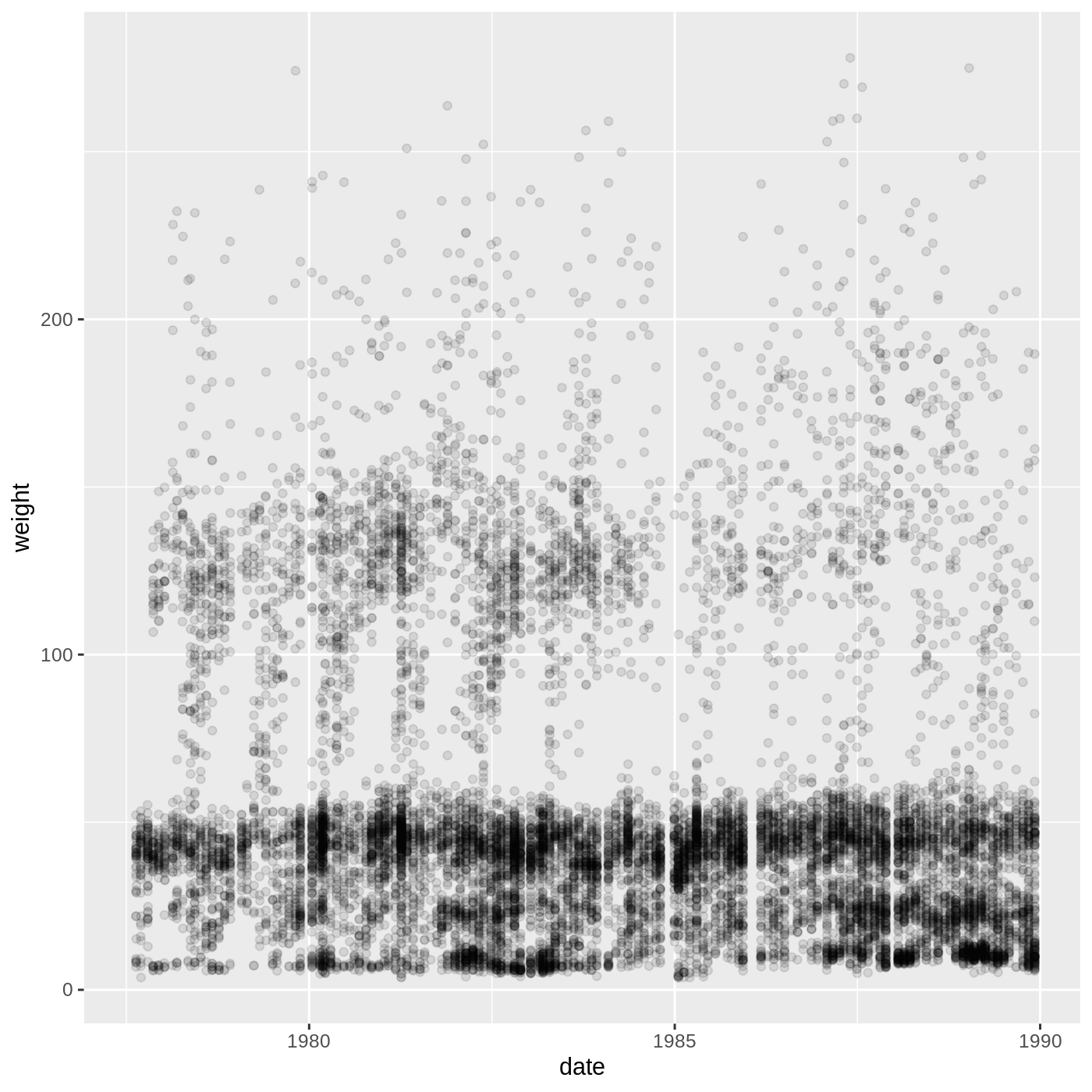
This isn’t necessarily the most useful plot, but we will learn some techniques that will help produce nice time series plots
The split-apply-combine approach
Many data analysis tasks can be achieved using the split-apply-combine approach: you split the data into groups, apply some analysis to each group, and combine the results in some way. dplyr has a few convenient functions to enable this approach, the main two being group_by() and summarize().
group_by() takes a data.frame and the name of one or more columns with categorical values that define the groups. summarize() then collapses each group into a one-row summary of the group, giving you back a data.frame with one row per group. The syntax for summarize() is similar to mutate(), where you define new columns based on values of other columns. Let’s try calculating the mean weight of all our animals by sex.
R
surveys %>%
  group_by(sex) %>%
  summarize(mean_weight = mean(weight, na.rm = T))
OUTPUT
# A tibble: 3 × 2
  sex   mean_weight
  <chr>       <dbl>
1 F            53.1
2 M            53.2
3 <NA>         74.0
You can see that the mean weight for males is slightly higher than for females, but that animals whose sex is unknown have much higher weights. This is probably due to small sample size, but we should check to be sure. Like mutate(), we can define multiple columns in one summarize() call. The function n() will count the number of rows in each group.
R
surveys %>%
  group_by(sex) %>%
  summarize(mean_weight = mean(weight, na.rm = T),
            n = n())
OUTPUT
# A tibble: 3 × 3
  sex   mean_weight     n
  <chr>       <dbl> <int>
1 F            53.1  7318
2 M            53.2  8260
3 <NA>         74.0  1300
You will often want to create groups based on multiple columns. For example, we might be interested in the mean weight of every species + sex combination. All we have to do is add another column to our group_by() call.
R
surveys %>%
  group_by(species_id, sex) %>%
  summarize(mean_weight = mean(weight, na.rm = T),
            n = n())
OUTPUT
`summarise()` has grouped output by 'species_id'. You can override using the
`.groups` argument.
OUTPUT
# A tibble: 67 × 4
# Groups:   species_id [36]
   species_id sex   mean_weight     n
   <chr>      <chr>       <dbl> <int>
 1 AB         <NA>        NaN     223
 2 AH         <NA>        NaN     136
 3 BA         M             7       3
 4 CB         <NA>        NaN      23
 5 CM         <NA>        NaN      13
 6 CQ         <NA>        NaN      16
 7 CS         <NA>        NaN       1
 8 CV         <NA>        NaN       1
 9 DM         F            40.7  2522
10 DM         M            44.0  3108
# … with 57 more rows
Our resulting data.frame is much larger, since we have a greater number of groups. We also see a strange value showing up in our mean_weight column: NaN. This stands for “Not a Number”, and it often results from trying to do an operation a vector with zero entries. How can a vector have zero entries? Well, if a particular group (like the AB species ID + NA sex group) has only NA values for weight, then the na.rm = T argument in mean() will remove all the values prior to calculating the mean. The result will be a value of NaN. Since we are not particularly interested in these values, let’s add a step to our pipeline to remove rows where weight is NA before doing any other steps. This means that any groups with only NA values will disappear from our data.frame before we formally create the groups with group_by().
R
surveys %>%
  filter(!is.na(weight)) %>%
  group_by(species_id, sex) %>%
  summarize(mean_weight = mean(weight),
            n = n())
OUTPUT
`summarise()` has grouped output by 'species_id'. You can override using the
`.groups` argument.
OUTPUT
# A tibble: 46 × 4
# Groups:   species_id [18]
   species_id sex   mean_weight     n
   <chr>      <chr>       <dbl> <int>
 1 BA         M             7       3
 2 DM         F            40.7  2460
 3 DM         M            44.0  3013
 4 DM         <NA>         37       8
 5 DO         F            48.4   679
 6 DO         M            49.3   748
 7 DO         <NA>         44       1
 8 DS         F           118.   1055
 9 DS         M           123.   1184
10 DS         <NA>        121.     16
# … with 36 more rows
That looks better! It’s often useful to take a look at the results in some order, like the lowest mean weight to highest. We can use the arrange() function for that:
R
surveys %>%
  filter(!is.na(weight)) %>%
  group_by(species_id, sex) %>%
  summarize(mean_weight = mean(weight),
            n = n()) %>%
  arrange(mean_weight)
OUTPUT
`summarise()` has grouped output by 'species_id'. You can override using the
`.groups` argument.
OUTPUT
# A tibble: 46 × 4
# Groups:   species_id [18]
   species_id sex   mean_weight     n
   <chr>      <chr>       <dbl> <int>
 1 PF         <NA>         6        2
 2 BA         M            7        3
 3 PF         F            7.09   215
 4 PF         M            7.10   296
 5 RM         M            9.92   678
 6 RM         <NA>        10.4      7
 7 RM         F           10.7    629
 8 RF         M           12.4     16
 9 RF         F           13.7     46
10 PP         <NA>        15        2
# … with 36 more rows
If we want to reverse the order, we can wrap the column name in desc():
R
surveys %>%
  filter(!is.na(weight)) %>%
  group_by(species_id, sex) %>%
  summarize(mean_weight = mean(weight),
            n = n()) %>%
  arrange(desc(mean_weight))
OUTPUT
`summarise()` has grouped output by 'species_id'. You can override using the
`.groups` argument.
OUTPUT
# A tibble: 46 × 4
# Groups:   species_id [18]
   species_id sex   mean_weight     n
   <chr>      <chr>       <dbl> <int>
 1 NL         M           168.    355
 2 NL         <NA>        164.      9
 3 NL         F           151.    460
 4 SS         M           130       1
 5 DS         M           123.   1184
 6 DS         <NA>        121.     16
 7 DS         F           118.   1055
 8 SH         F            79.2    61
 9 SH         M            67.6    34
10 SF         F            58.3     3
# … with 36 more rows
You may have seen several messages saying summarise() has grouped output by 'species_id'. You can override using the .groups argument. These are warning you that your resulting data.frame has retained some group structure, which means any subsequent operations on that data.frame will happen at the group level. If you look at the resulting data.frame printed out in your console, you will see these lines:
# A tibble: 46 × 4
# Groups:   species_id [18]
They tell us we have a data.frame with 46 rows, 4 columns, and a group variable species_id, for which there are 18 groups. We will see something similar if we use group_by() alone:
R
surveys %>%
  group_by(species_id, sex)
OUTPUT
# A tibble: 16,878 × 13
# Groups:   species_id, sex [67]
   record_id month   day  year plot_id species_id sex   hindfoot_length weight
       <dbl> <dbl> <dbl> <dbl>   <dbl> <chr>      <chr>           <dbl>  <dbl>
 1         1     7    16  1977       2 NL         M                  32     NA
 2         2     7    16  1977       3 NL         M                  33     NA
 3         3     7    16  1977       2 DM         F                  37     NA
 4         4     7    16  1977       7 DM         M                  36     NA
 5         5     7    16  1977       3 DM         M                  35     NA
 6         6     7    16  1977       1 PF         M                  14     NA
 7         7     7    16  1977       2 PE         F                  NA     NA
 8         8     7    16  1977       1 DM         M                  37     NA
 9         9     7    16  1977       1 DM         F                  34     NA
10        10     7    16  1977       6 PF         F                  20     NA
# … with 16,868 more rows, and 4 more variables: genus <chr>, species <chr>,
#   taxa <chr>, plot_type <chr>
What we get back is the entire surveys data.frame, but with the grouping variables added: 67 groups of species_id + sex combinations. Groups are often maintained throughout a pipeline, and if you assign the resulting data.frame to a new object, it will also have those groups. This can lead to confusing results if you forget about the grouping and want to carry out operations on the whole data.frame, not by group. Therefore, it is a good habit to remove the groups at the end of a pipeline containing group_by():
R
surveys %>%
  filter(!is.na(weight)) %>%
  group_by(species_id, sex) %>%
  summarize(mean_weight = mean(weight),
            n = n()) %>%
  arrange(desc(mean_weight)) %>%
  ungroup()
OUTPUT
`summarise()` has grouped output by 'species_id'. You can override using the
`.groups` argument.
OUTPUT
# A tibble: 46 × 4
   species_id sex   mean_weight     n
   <chr>      <chr>       <dbl> <int>
 1 NL         M           168.    355
 2 NL         <NA>        164.      9
 3 NL         F           151.    460
 4 SS         M           130       1
 5 DS         M           123.   1184
 6 DS         <NA>        121.     16
 7 DS         F           118.   1055
 8 SH         F            79.2    61
 9 SH         M            67.6    34
10 SF         F            58.3     3
# … with 36 more rows
Now our data.frame just says # A tibble: 46 × 4 at the top, with no groups.
While it is common that you will want to get the one-row-per-group summary that summarise() provides, there are times where you want to calculate a per-group value but keep all the rows in your data.frame. For example, we might want to know the mean weight for each species ID + sex combination, and then we might want to know how far from that mean value each observation in the group is. For this, we can use group_by() and mutate() together:
R
surveys %>%
  filter(!is.na(weight)) %>%
  group_by(species_id, sex) %>%
  mutate(mean_weight = mean(weight),
            weight_diff = weight - mean_weight)
OUTPUT
# A tibble: 15,186 × 15
# Groups:   species_id, sex [46]
   record_id month   day  year plot_id species_id sex   hindfoot_length weight
       <dbl> <dbl> <dbl> <dbl>   <dbl> <chr>      <chr>           <dbl>  <dbl>
 1        63     8    19  1977       3 DM         M                  35     40
 2        64     8    19  1977       7 DM         M                  37     48
 3        65     8    19  1977       4 DM         F                  34     29
 4        66     8    19  1977       4 DM         F                  35     46
 5        67     8    19  1977       7 DM         M                  35     36
 6        68     8    19  1977       8 DO         F                  32     52
 7        69     8    19  1977       2 PF         M                  15      8
 8        70     8    19  1977       3 OX         F                  21     22
 9        71     8    19  1977       7 DM         F                  36     35
10        74     8    19  1977       8 PF         M                  12      7
# … with 15,176 more rows, and 6 more variables: genus <chr>, species <chr>,
#   taxa <chr>, plot_type <chr>, mean_weight <dbl>, weight_diff <dbl>
Since we get all our columns back, the new columns are at the very end and don’t print out in the console. Let’s use select() to just look at the columns of interest. Inside select() we can use the contains() function to get any column containing the word “weight” in the name:
R
surveys %>%
  filter(!is.na(weight)) %>%
  group_by(species_id, sex) %>%
  mutate(mean_weight = mean(weight),
            weight_diff = weight - mean_weight) %>%
  select(species_id, sex, contains("weight"))
OUTPUT
# A tibble: 15,186 × 5
# Groups:   species_id, sex [46]
   species_id sex   weight mean_weight weight_diff
   <chr>      <chr>  <dbl>       <dbl>       <dbl>
 1 DM         M         40       44.0      -4.00
 2 DM         M         48       44.0       4.00
 3 DM         F         29       40.7     -11.7
 4 DM         F         46       40.7       5.28
 5 DM         M         36       44.0      -8.00
 6 DO         F         52       48.4       3.63
 7 PF         M          8        7.10      0.902
 8 OX         F         22       21         1
 9 DM         F         35       40.7      -5.72
10 PF         M          7        7.10     -0.0980
# … with 15,176 more rows
What happens with the group_by() + mutate() combination is similar to using summarize(): for each group, the mean weight is calculated. However, instead of reporting only one row per group, the mean weight for each group is added to each row in that group. For each row in a group (like DM species ID + M sex), you will see the same value in mean_weight.
R
surveys_daily_counts <- surveys %>%
  mutate(date = ymd(paste(year, month, day, sep = "-"))) %>%
  group_by(date, sex) %>%
  summarize(n = n())
OUTPUT
`summarise()` has grouped output by 'date'. You can override using the
`.groups` argument.
R
# shorter approach using count()
surveys_daily_counts <- surveys %>%
  mutate(date = ymd(paste(year, month, day, sep = "-"))) %>%
  count(date, sex)
Challenge 4: Making a time series (continued)
- Now use the data.frame you just made to plot the daily number of animals of each sex caught over time. It’s up to you what
geomto use, but alineplot might be a good choice. You should also think about how to differentiate which data corresponds to which sex.
R
surveys_daily_counts %>%
  ggplot(aes(x = date, y = n, color = sex)) +
  geom_line()
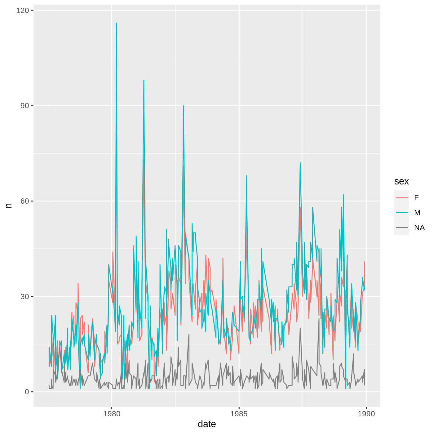
Reshaping data with tidyr
Let’s say we are interested in comparing the mean weights of each species across our different plots. We can begin this process using the group_by() + summarize() approach:
R
sp_by_plot <- surveys %>%
  filter(!is.na(weight)) %>%
  group_by(species_id, plot_id) %>%
  summarise(mean_weight = mean(weight)) %>%
  arrange(species_id, plot_id)
OUTPUT
`summarise()` has grouped output by 'species_id'. You can override using the
`.groups` argument.
R
sp_by_plot
OUTPUT
# A tibble: 300 × 3
# Groups:   species_id [18]
   species_id plot_id mean_weight
   <chr>        <dbl>       <dbl>
 1 BA               3         8
 2 BA              21         6.5
 3 DM               1        42.7
 4 DM               2        42.6
 5 DM               3        41.2
 6 DM               4        41.9
 7 DM               5        42.6
 8 DM               6        42.1
 9 DM               7        43.2
10 DM               8        43.4
# … with 290 more rows
That looks great, but it is a bit difficult to compare values across plots. It would be nice if we could reshape this data.frame to make those comparisons easier. Well, the tidyr package from the tidyverse has a pair of functions that allow you to reshape data by pivoting it: pivot_wider() and pivot_longer(). pivot_wider() will make the data wider, which means increasing the number of columns and reducing the number of rows. pivot_longer() will do the opposite, reducing the number of columns and increasing the number of rows.
In this case, it might be nice to create a data.frame where each species has its own row, and each plot has its own column containing the mean weight for a given species. We will use pivot_wider() to reshape our data in this way. It takes 3 arguments:
- the name of the data.frame
-
names_from: which column should be used to generate the names of the new columns? -
values_from: which column should be used to fill in the values of the new columns?
Any columns not used for names_from or values_from will not be pivoted.
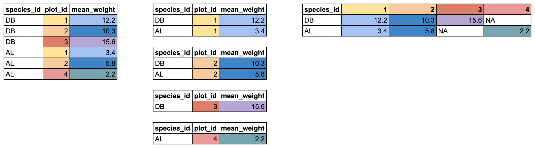
In our case, we want the new columns to be named from our plot_id column, with the values coming from the mean_weight column. We can pipe our data.frame right into pivot_wider() and add those two arguments:
R
sp_by_plot_wide <- sp_by_plot %>%
  pivot_wider(names_from = plot_id,
              values_from = mean_weight)

sp_by_plot_wide
OUTPUT
# A tibble: 18 × 25
# Groups:   species_id [18]
   species_id    `3`   `21`    `1`    `2`    `4`   `5`    `6`   `7`    `8`
   <chr>       <dbl>  <dbl>  <dbl>  <dbl>  <dbl> <dbl>  <dbl> <dbl>  <dbl>
 1 BA           8      6.5   NA     NA     NA     NA    NA     NA    NA
 2 DM          41.2   41.5   42.7   42.6   41.9   42.6  42.1   43.2  43.4
 3 DO          42.7   NA     50.1   50.3   46.8   50.4  49.0   52    49.2
 4 DS         128.    NA    129.   125.   118.   111.  114.   126.  128.
 5 NL         171.   136.   154.   171.   164.   192.  176.   170.  134.
 6 OL          32.1   28.6   35.5   34     33.0   32.6  31.8   NA    30.3
 7 OT          24.1   24.1   23.7   24.9   26.5   23.6  23.5   22    24.1
 8 OX          22     NA     NA     22     NA     20    NA     NA    NA
 9 PE          22.7   19.6   21.6   22.0   NA     21    21.6   22.8  19.4
10 PF           7.12   7.23   6.57   6.89   6.75   7.5   7.54   7     6.78
11 PH          28     31     NA     NA     NA     29    NA     NA    NA
12 PM          20.1   23.6   23.7   23.9   NA     23.7  22.3   23.4  23
13 PP          17.1   13.6   14.3   16.4   14.8   19.8  16.8   NA    13.9
14 RF          14.8   17     NA     16     NA     14    12.1   13    NA
15 RM          10.3    9.89  10.9   10.6   10.4   10.8  10.6   10.7   9
16 SF          NA     49     NA     NA     NA     NA    NA     NA    NA
17 SH          76.0   79.9   NA     88     NA     82.7  NA     NA    NA
18 SS          NA     NA     NA     NA     NA     NA    NA     NA    NA
# … with 15 more variables: `9` <dbl>, `10` <dbl>, `11` <dbl>, `12` <dbl>,
#   `13` <dbl>, `14` <dbl>, `15` <dbl>, `16` <dbl>, `17` <dbl>, `18` <dbl>,
#   `19` <dbl>, `20` <dbl>, `22` <dbl>, `23` <dbl>, `24` <dbl>
Now we’ve got our reshaped data.frame. There are a few things to notice. First, we have a new column for each plot_id value. There is one old column left in the data.frame: species_id. It wasn’t used in pivot_wider(), so it stays, and now contains a single entry for each unique species_id value.
Finally, a lot of NAs have appeared. Some species aren’t found in every plot, but because a data.frame has to have a value in every row and every column, an NA is inserted. We can double-check this to verify what is going on.
Looking in our new pivoted data.frame, we can see that there is an NA value for the species BA in plot 1. Let’s take our sp_by_plot data.frame and look for the mean_weight of that species + plot combination.
R
sp_by_plot %>%
  filter(species_id == "BA" & plot_id == 1)
OUTPUT
# A tibble: 0 × 3
# Groups:   species_id [0]
# … with 3 variables: species_id <chr>, plot_id <dbl>, mean_weight <dbl>
We get back 0 rows. There is no mean_weight for the species BA in plot 1. This either happened because no BA were ever caught in plot 1, or because every BA caught in plot 1 had an NA weight value and all the rows got removed when we used filter(!is.na(weight)) in the process of making sp_by_plot. Because there are no rows with that species + plot combination, in our pivoted data.frame, the value gets filled with NA.
There is another pivot_ function that does the opposite, moving data from a wide to long format, called pivot_longer(). It takes 3 arguments: cols for the columns you want to pivot, names_to for the name of the new column which will contain the old column names, and values_to for the name of the new column which will contain the old values.
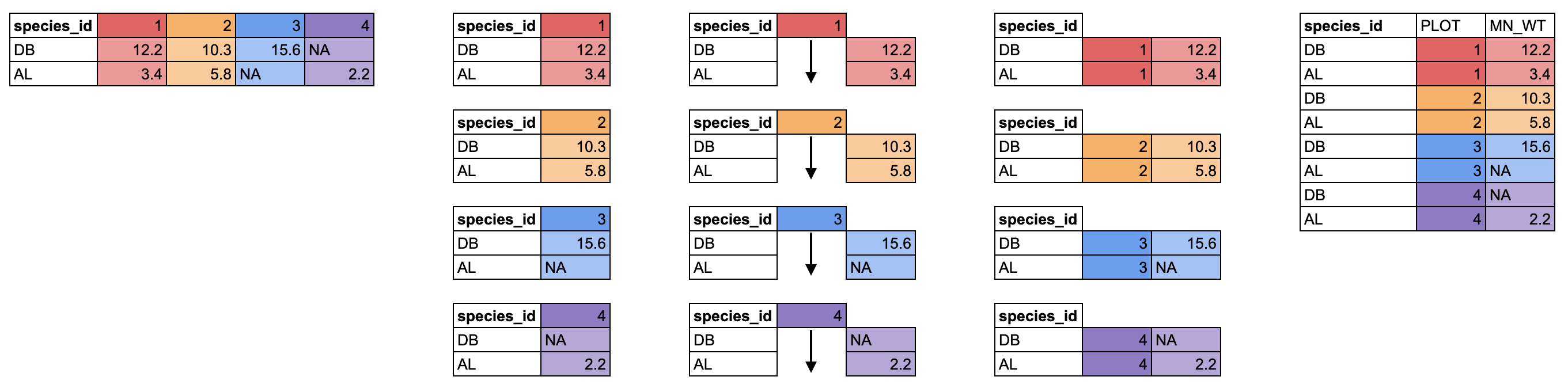
We can pivot our new wide data.frame to a long format using pivot_longer(). We want to pivot all the columns except species_id, and we will use PLOT for the new column of plot IDs, and MEAN_WT for the new column of mean weight values.
R
sp_by_plot_wide %>%
  pivot_longer(cols = -species_id, names_to = "PLOT", values_to = "MEAN_WT")
OUTPUT
# A tibble: 432 × 3
# Groups:   species_id [18]
   species_id PLOT  MEAN_WT
   <chr>      <chr>   <dbl>
 1 BA         3         8
 2 BA         21        6.5
 3 BA         1        NA
 4 BA         2        NA
 5 BA         4        NA
 6 BA         5        NA
 7 BA         6        NA
 8 BA         7        NA
 9 BA         8        NA
10 BA         9        NA
# … with 422 more rows
One thing you will notice is that all those NA values that got generated when we pivoted wider. However, we can filter those out, which gets us back to the same data as sp_by_plot, before we pivoted it wider.
R
sp_by_plot_wide %>%
  pivot_longer(cols = -species_id, names_to = "PLOT", values_to = "MEAN_WT") %>%
  filter(!is.na(MEAN_WT))
OUTPUT
# A tibble: 300 × 3
# Groups:   species_id [18]
   species_id PLOT  MEAN_WT
   <chr>      <chr>   <dbl>
 1 BA         3         8
 2 BA         21        6.5
 3 DM         3        41.2
 4 DM         21       41.5
 5 DM         1        42.7
 6 DM         2        42.6
 7 DM         4        41.9
 8 DM         5        42.6
 9 DM         6        42.1
10 DM         7        43.2
# … with 290 more rows
Data are often recorded in spreadsheets in a wider format, but lots of tidyverse tools, especially ggplot2, like data in a longer format, so pivot_longer() is often very useful.
Exporting data
Let’s say we want to send the wide version of our sb_by_plot data.frame to a colleague who doesn’t use R. In this case, we might want to save it as a CSV file.
First, we might want to modify the names of the columns, since right now they are bare numbers, which aren’t very informative. Luckily, pivot_wider() has an argument names_prefix which will allow us to add “plot_” to the start of each column.
R
sp_by_plot %>%
  pivot_wider(names_from = plot_id, values_from = mean_weight,
              names_prefix = "plot_")
OUTPUT
# A tibble: 18 × 25
# Groups:   species_id [18]
   species_id plot_3 plot_21 plot_1 plot_2 plot_4 plot_5 plot_6 plot_7 plot_8
   <chr>       <dbl>   <dbl>  <dbl>  <dbl>  <dbl>  <dbl>  <dbl>  <dbl>  <dbl>
 1 BA           8       6.5   NA     NA     NA      NA    NA      NA    NA
 2 DM          41.2    41.5   42.7   42.6   41.9    42.6  42.1    43.2  43.4
 3 DO          42.7    NA     50.1   50.3   46.8    50.4  49.0    52    49.2
 4 DS         128.     NA    129.   125.   118.    111.  114.    126.  128.
 5 NL         171.    136.   154.   171.   164.    192.  176.    170.  134.
 6 OL          32.1    28.6   35.5   34     33.0    32.6  31.8    NA    30.3
 7 OT          24.1    24.1   23.7   24.9   26.5    23.6  23.5    22    24.1
 8 OX          22      NA     NA     22     NA      20    NA      NA    NA
 9 PE          22.7    19.6   21.6   22.0   NA      21    21.6    22.8  19.4
10 PF           7.12    7.23   6.57   6.89   6.75    7.5   7.54    7     6.78
11 PH          28      31     NA     NA     NA      29    NA      NA    NA
12 PM          20.1    23.6   23.7   23.9   NA      23.7  22.3    23.4  23
13 PP          17.1    13.6   14.3   16.4   14.8    19.8  16.8    NA    13.9
14 RF          14.8    17     NA     16     NA      14    12.1    13    NA
15 RM          10.3     9.89  10.9   10.6   10.4    10.8  10.6    10.7   9
16 SF          NA      49     NA     NA     NA      NA    NA      NA    NA
17 SH          76.0    79.9   NA     88     NA      82.7  NA      NA    NA
18 SS          NA      NA     NA     NA     NA      NA    NA      NA    NA
# … with 15 more variables: plot_9 <dbl>, plot_10 <dbl>, plot_11 <dbl>,
#   plot_12 <dbl>, plot_13 <dbl>, plot_14 <dbl>, plot_15 <dbl>, plot_16 <dbl>,
#   plot_17 <dbl>, plot_18 <dbl>, plot_19 <dbl>, plot_20 <dbl>, plot_22 <dbl>,
#   plot_23 <dbl>, plot_24 <dbl>
That looks better! Let’s save this data.frame as a new object.
R
surveys_sp <- sp_by_plot %>%
  pivot_wider(names_from = plot_id, values_from = mean_weight,
              names_prefix = "plot_")

surveys_sp
OUTPUT
# A tibble: 18 × 25
# Groups:   species_id [18]
   species_id plot_3 plot_21 plot_1 plot_2 plot_4 plot_5 plot_6 plot_7 plot_8
   <chr>       <dbl>   <dbl>  <dbl>  <dbl>  <dbl>  <dbl>  <dbl>  <dbl>  <dbl>
 1 BA           8       6.5   NA     NA     NA      NA    NA      NA    NA
 2 DM          41.2    41.5   42.7   42.6   41.9    42.6  42.1    43.2  43.4
 3 DO          42.7    NA     50.1   50.3   46.8    50.4  49.0    52    49.2
 4 DS         128.     NA    129.   125.   118.    111.  114.    126.  128.
 5 NL         171.    136.   154.   171.   164.    192.  176.    170.  134.
 6 OL          32.1    28.6   35.5   34     33.0    32.6  31.8    NA    30.3
 7 OT          24.1    24.1   23.7   24.9   26.5    23.6  23.5    22    24.1
 8 OX          22      NA     NA     22     NA      20    NA      NA    NA
 9 PE          22.7    19.6   21.6   22.0   NA      21    21.6    22.8  19.4
10 PF           7.12    7.23   6.57   6.89   6.75    7.5   7.54    7     6.78
11 PH          28      31     NA     NA     NA      29    NA      NA    NA
12 PM          20.1    23.6   23.7   23.9   NA      23.7  22.3    23.4  23
13 PP          17.1    13.6   14.3   16.4   14.8    19.8  16.8    NA    13.9
14 RF          14.8    17     NA     16     NA      14    12.1    13    NA
15 RM          10.3     9.89  10.9   10.6   10.4    10.8  10.6    10.7   9
16 SF          NA      49     NA     NA     NA      NA    NA      NA    NA
17 SH          76.0    79.9   NA     88     NA      82.7  NA      NA    NA
18 SS          NA      NA     NA     NA     NA      NA    NA      NA    NA
# … with 15 more variables: plot_9 <dbl>, plot_10 <dbl>, plot_11 <dbl>,
#   plot_12 <dbl>, plot_13 <dbl>, plot_14 <dbl>, plot_15 <dbl>, plot_16 <dbl>,
#   plot_17 <dbl>, plot_18 <dbl>, plot_19 <dbl>, plot_20 <dbl>, plot_22 <dbl>,
#   plot_23 <dbl>, plot_24 <dbl>
Now we can save this data.frame to a CSV using the write_csv() function from the readr package. The first argument is the name of the data.frame, and the second is the path to the new file we want to create, including the file extension .csv.
R
write_csv(surveys_sp, "data/cleaned/surveys_meanweight_species_plot.csv")
If we go look into our data/cleaned_data folder, we will see this new CSV file.
Keypoints
- use
filter()to subset rows andselect()to subset columns - build up pipelines one step at a time before assigning the result
- it is often best to keep components of dates separate until needed, then use
mutate()to make a date column -
group_by()can be used withsummarize()to collapse rows ormutate()to keep the same number of rows -
pivot_wider()andpivot_longer()are powerful for reshaping data, but you should plan out how to use them thoughtfully
Content from Putting it together
Last updated on 2022-11-29 | Edit this page
Overview
Questions
- How do you apply data manipulation skills to multiple new files?
Objectives
- Read in messy data and find issues.
- Replace incorrect values.
- Read data from multiple file formats.
- Utilize
pivot_functions to reshape untidy data. - Combine multiple datasets.
- Understand the process of formatting new data similarly to existing data.
R
library(tidyverse)
So far we have been working with surveys data from 1977 to 1989, and our data have been pretty neat and tidy. There are some NA values, but for the most part, the data have been formatted nicely. However, as many of us know, we do not always receive data in such nice shape. It’s pretty common to get data with all sorts of formatting issues, maybe some strange file formats, and possibly spread across several different sources.
Well, it turns out we have just that situation! We have received a newer batch of surveys data, from 1990 to 2002, and we want to add it to our older dataset so we can work with them together. Unfortunately, the data are not formatted quite as nicely as our old data. Our collaborators have told us to “look them over” for any errors, but have not given us very much specific information. We will have to explore the new data to make sure we understand it and verify that there aren’t any errors.
You can download a .zip file containing three new data files here: https://www.michaelc-m.com/Rewrite-R-ecology-lesson/data/new_data.zip. When prompted, save the file to your data/raw/ folder. A .zip file is a type of compressed file that contains one or more files or directories. We will use the unzip() command to extract the data files from the .zip file. The first argument is the path to the .zip file, the next argument is the directory we want to put the extracted files into, and the last argument tells unzip() to not create an additional directory for the new files. Since this is an action we only want to perform once, we will run it directly in the Console instead of putting it into a script.
R
unzip("data/raw/new_data.zip", exdir = "data/raw/", junkpaths = TRUE)
Use the Files pane in the lower right to navigate to the data/raw/ folder and you should find 3 new files: plots_new.csv, species_new.txt, and surveys_new.csv.
Reading the new surveys data
Let’s start off with the new surveys data. First we will read it into R:
R
surveys_new <- read_csv("data/raw/surveys_new.csv")
WARNING
Warning: One or more parsing issues, see `problems()` for detailsOUTPUT
Rows: 18676 Columns: 7
── Column specification ────────────────────────────────────────────────────────
Delimiter: ","
chr (3): date (mm/dd/yyyy), species_id, sex
dbl (4): record_id, plot_id, hindfoot_length, weight

ℹ Use `spec()` to retrieve the full column specification for this data.
ℹ Specify the column types or set `show_col_types = FALSE` to quiet this message.
You will notice it contains a lot of columns from our previous surveys data, but not all of the columns. Some of them are only found in our other plots_new.csv and species_new.txt files.
First thing we want to do with surveys_new is fix that date column name with spaces in it. R can handle them, but they are often very annoying. We can use the rename() function to change the column name.
R
surveys_new <- surveys_new %>%
  rename(date = `date (mm/dd/yyyy)`)
Let’s take a look at a summary of our data using summary().
R
summary(surveys_new)
OUTPUT
   record_id         date              plot_id       species_id
 Min.   :16879   Length:18676       Min.   : 1.00   Length:18676
 1st Qu.:21545   Class :character   1st Qu.: 5.00   Class :character
 Median :26214   Mode  :character   Median :12.00   Mode  :character
 Mean   :26214                      Mean   :11.33
 3rd Qu.:30881                      3rd Qu.:17.00
 Max.   :35549                      Max.   :24.00

     sex            hindfoot_length     weight
 Length:18676       Min.   : 2.00   Min.   :   4.0
 Class :character   1st Qu.:21.00   1st Qu.:  19.0
 Mode  :character   Median :26.00   Median :  32.0
                    Mean   :27.08   Mean   : 873.7
                    3rd Qu.:36.00   3rd Qu.:  47.0
                    Max.   :64.00   Max.   :9999.0
                    NA's   :1380
The summary() function is often useful for detecting outliers or clearly incorrect values, since we get a Min. and Max. value for each numeric column. For example, we see that month goes from 1 to 12 and day goes from 1 to 31, so no issues there. However, we do notice that weight has a max value of 9999. Sometimes people will use extreme and impossible values to denote a missing value. It is worth checking with our collaborators to make sure this is the case, but we will assume that’s what happened.
Finally, we actually got a warning message about a parsing issue. This message actually comes from read_csv(), even though it only showed up now. Parsing is what read_csv() does when it tries to guess what type of vector each CSV column should be. Sometimes it will warn us about issues that occurred, which we can then investigate with the problems() function.
R
problems(surveys_new)
OUTPUT
# A tibble: 1 × 5
    row   col expected actual file
  <int> <int> <chr>    <chr>  <chr>
1    19     6 a double 19'    /home/runner/work/Rewrite-R-ecology-lesson/Rewrit…
The output shows that in the 19th row and 8th column of the CSV, read_csv() expected a double, or numeric, value. Instead, what it got was 19'. That stray quotation mark was unexpected, so read_csv() notified us. Let’s go see what value is actually there for surveys_new. It was in the 19th row of the CSV, which includes the header row containing column names, so we should look at the 18th row of our data.frame. The 8th column is hindfoot_length. We can use the head() function to look at the first 20 rows.
R
surveys_new %>%
  head(n=20)
OUTPUT
# A tibble: 20 × 7
   record_id date     plot_id species_id sex   hindfoot_length weight
       <dbl> <chr>      <dbl> <chr>      <chr>           <dbl>  <dbl>
 1     16879 1/6/1990       1 DM         F                  37     35
 2     16880 1/6/1990       1 OL         M                  21     28
 3     16881 1/6/1990       6 PF         M                  16      7
 4     16882 1/6/1990      23 RM         F                  17      9
 5     16883 1/6/1990      12 RM         M                  17     10
 6     16884 1/6/1990      24 RM         M                  17      9
 7     16885 1/6/1990      12 SF         M                  25     35
 8     16886 1/6/1990      24 SH         F                  30     73
 9     16887 1/6/1990      12 SF         M                  28     44
10     16888 1/6/1990      17 DO         M                  36     55
11     16889 1/6/1990      21 SF         M                  29     55
12     16890 1/6/1990      12 OT         M                  22     23
13     16891 1/6/1990      12 DO         F                  36     53
14     16892 1/6/1990      21 AB         <NA>               NA   9999
15     16893 1/6/1990      12 OT         F                  21     24
16     16894 1/6/1990       1 OT         F                  21     20
17     16895 1/6/1990      12 SF         F                  27     75
18     16896 1/6/1990      12 RM         M                  NA     11
19     16897 1/6/1990      21 SF         F                  29     46
20     16898 1/6/1990      23 RM         M                  18     11
Because read_csv() didn’t know what to do with the value 19', there is an NA for hindfoot_length in row 18. It is likely that the true value was 19 and the stray quotation mark was simply a typo. If we want to change that value, we can do it by referring to the record_id, since it is a unique identifier for each row. We will use the function if_else() to actually replace the value. This function takes a logical statement as its first argument, then a value to return if that statement is TRUE, and a value to return if it is FALSE. Take a look at this example:
R
x <- 1:10
ifelse(x > 6, "bigger than 6", "not bigger than 6")
OUTPUT
 [1] "not bigger than 6" "not bigger than 6" "not bigger than 6"
 [4] "not bigger than 6" "not bigger than 6" "not bigger than 6"
 [7] "bigger than 6"     "bigger than 6"     "bigger than 6"
[10] "bigger than 6"
What we will do is take surveys_new and mutate the hindfoot_length column. It will be equal to the result of an ifelse() statement. If the record_id is 16896, the row we are trying to change, then hindfoot_length will be set to 19. If the record_id is not 16896, then it will stay as the current hindfoot_length value.
R
surveys_new <- surveys_new %>%
  mutate(hindfoot_length = ifelse(record_id == 16896, 19, hindfoot_length))

surveys_new %>%
  head(n=20)
OUTPUT
# A tibble: 20 × 7
   record_id date     plot_id species_id sex   hindfoot_length weight
       <dbl> <chr>      <dbl> <chr>      <chr>           <dbl>  <dbl>
 1     16879 1/6/1990       1 DM         F                  37     35
 2     16880 1/6/1990       1 OL         M                  21     28
 3     16881 1/6/1990       6 PF         M                  16      7
 4     16882 1/6/1990      23 RM         F                  17      9
 5     16883 1/6/1990      12 RM         M                  17     10
 6     16884 1/6/1990      24 RM         M                  17      9
 7     16885 1/6/1990      12 SF         M                  25     35
 8     16886 1/6/1990      24 SH         F                  30     73
 9     16887 1/6/1990      12 SF         M                  28     44
10     16888 1/6/1990      17 DO         M                  36     55
11     16889 1/6/1990      21 SF         M                  29     55
12     16890 1/6/1990      12 OT         M                  22     23
13     16891 1/6/1990      12 DO         F                  36     53
14     16892 1/6/1990      21 AB         <NA>               NA   9999
15     16893 1/6/1990      12 OT         F                  21     24
16     16894 1/6/1990       1 OT         F                  21     20
17     16895 1/6/1990      12 SF         F                  27     75
18     16896 1/6/1990      12 RM         M                  19     11
19     16897 1/6/1990      21 SF         F                  29     46
20     16898 1/6/1990      23 RM         M                  18     11
We can actually use ifelse() to fix the values of 9999 in the weight column as well.
R
surveys_new <- surveys_new %>%
  mutate(weight = ifelse(weight == 9999, NA, weight))

surveys_new %>%
  head(n=20)
OUTPUT
# A tibble: 20 × 7
   record_id date     plot_id species_id sex   hindfoot_length weight
       <dbl> <chr>      <dbl> <chr>      <chr>           <dbl>  <dbl>
 1     16879 1/6/1990       1 DM         F                  37     35
 2     16880 1/6/1990       1 OL         M                  21     28
 3     16881 1/6/1990       6 PF         M                  16      7
 4     16882 1/6/1990      23 RM         F                  17      9
 5     16883 1/6/1990      12 RM         M                  17     10
 6     16884 1/6/1990      24 RM         M                  17      9
 7     16885 1/6/1990      12 SF         M                  25     35
 8     16886 1/6/1990      24 SH         F                  30     73
 9     16887 1/6/1990      12 SF         M                  28     44
10     16888 1/6/1990      17 DO         M                  36     55
11     16889 1/6/1990      21 SF         M                  29     55
12     16890 1/6/1990      12 OT         M                  22     23
13     16891 1/6/1990      12 DO         F                  36     53
14     16892 1/6/1990      21 AB         <NA>               NA     NA
15     16893 1/6/1990      12 OT         F                  21     24
16     16894 1/6/1990       1 OT         F                  21     20
17     16895 1/6/1990      12 SF         F                  27     75
18     16896 1/6/1990      12 RM         M                  19     11
19     16897 1/6/1990      21 SF         F                  29     46
20     16898 1/6/1990      23 RM         M                  18     11
Challenge 1: Find a specialized function
The tidyverse often has specialized functions for common data manipulation tasks, such as replacing a certain values with NA. There is a tidyverse function to replace a value in a vector with NA. Put your Googling skills to work and see if you can find the correct function.
For an extra challenge, write out code that could use this function to replace weight values of 9999 with NA.
The dplyr function na_if() will replace specific values in a vector to NA. To find this function, you can Google “tidyverse replace value with NA”. One of the first results is the dplyr documentation page for the na_if() function.
If you scroll down to the bottom section of the documentation, you will find several examples, including how to use the function inside mutate().
R
surveys_new %>%
  mutate(weight = na_if(weight, 9999))
The last thing we have to do is deal with our date column. It’s currently a character column, but our old surveys data had separate columns for year, month, and day. Another thing we should do is check for any errors in our dates, since they are an error-prone data type.
There are a few ways we could approach this problem, which is a common theme in R: there are often many ways to accomplish the same task. It is often useful to plan your approach ahead of time, so we will describe two possible methods:
Turn the current column into a date column, validate the dates, then use
lubridatefunctions to extract the year, month, and day into their own columns.Use the
separate()function to split our current date column into 3 new character columns, containing the month, day and year. Then turn those columns into numeric columns. Then it will match our oldsurveysdata, and we can later make a date column to validate our dates.
It is often useful to plan out your approach, or several approaches, before you start writing code. It can be in the form of plain English like above, or in “pseudo-code”, which is laid out like code, but doesn’t have explicit, functioning code.
We will go ahead and use the first approach. First we will load lubridate and use the mdy() function to turn our date column into a date instead of character column.
R
library(lubridate)
OUTPUT
Attaching package: 'lubridate'OUTPUT
The following objects are masked from 'package:base':

    date, intersect, setdiff, union
R
surveys_new <- surveys_new %>%
  mutate(date = mdy(date))
WARNING
Warning: 6 failed to parse.We got a warning message about 6 dates failing to parse. This means that the mdy() function encountered 6 dates that it wasn’t able to identify correctly. When lubridate functions fail to parse dates, they will return an NA value instead. To find the rows where this happened, we can use filter():
R
surveys_new %>%
  filter(is.na(date))
OUTPUT
# A tibble: 6 × 7
  record_id date   plot_id species_id sex   hindfoot_length weight
      <dbl> <date>   <dbl> <chr>      <chr>           <dbl>  <dbl>
1     22258 NA           8 AH         <NA>               NA     NA
2     22261 NA           9 DM         F                  37     45
3     30595 NA          18 PB         F                  25     34
4     30610 NA           2 PB         F                  25     31
5     30638 NA          20 PP         F                  22     20
6     31394 NA          12 OT         F                  20     29
Challenge 2: Find the bad dates
We have now located the rows with NA dates, but we probably want to know what the original date character strings looked like. Figure out what those dates were and why they might have been wrong.
Hint: you will have to look at a previous version of the data, before we modified the date column.
There are two basic approaches you could take. First, you could look directly at the old CSV and find the rows with bad dates based on their record_id.
You could also read the data back into R and use filter() to pick out those specific rows via record_id:
R
read_csv("data/raw/surveys_new.csv") %>%
  filter(record_id %in% c(22258, 22261, 30595, 30610, 30638, 31394))
WARNING
Warning: One or more parsing issues, see `problems()` for detailsOUTPUT
# A tibble: 6 × 7
  record_id `date (mm/dd/yyyy)` plot_id species_id sex   hindfoot_length weight
      <dbl> <chr>                 <dbl> <chr>      <chr>           <dbl>  <dbl>
1     22258 4/31/1995                 8 AH         <NA>               NA   9999
2     22261 4/31/1995                 9 DM         F                  37     45
3     30595 4/31/2000                18 PB         F                  25     34
4     30610 4/31/2000                 2 PB         F                  25     31
5     30638 4/31/2000                20 PP         F                  22     20
6     31394 9/31/2000                12 OT         F                  20     29
The dates are wrong because they are the 31st day in a month that only has 30 days, like April or September. lubridate doesn’t recognize these as valid dates. The same thing can happen with things like dates in February during non-leap years.
The last thing to do is extract the year, month, and day values from our date column. lubridate has functions to extract each component of a date. We will then get rid of the date column, since it doesn’t appear in our original surveys data, and we can always remake it from the component columns.
R
surveys_new <- surveys_new %>%
  mutate(year = year(date),
         month = month(date),
         day = day(date)) %>%
  select(-date)

surveys_new
OUTPUT
# A tibble: 18,676 × 9
   record_id plot_id species_id sex   hindfoot_length weight  year month   day
       <dbl>   <dbl> <chr>      <chr>           <dbl>  <dbl> <dbl> <dbl> <int>
 1     16879       1 DM         F                  37     35  1990     1     6
 2     16880       1 OL         M                  21     28  1990     1     6
 3     16881       6 PF         M                  16      7  1990     1     6
 4     16882      23 RM         F                  17      9  1990     1     6
 5     16883      12 RM         M                  17     10  1990     1     6
 6     16884      24 RM         M                  17      9  1990     1     6
 7     16885      12 SF         M                  25     35  1990     1     6
 8     16886      24 SH         F                  30     73  1990     1     6
 9     16887      12 SF         M                  28     44  1990     1     6
10     16888      17 DO         M                  36     55  1990     1     6
# … with 18,666 more rows
Reading the new species data
Our surveys_new data look good at this point, so let’s move on to the species data. You may have noticed that our species data came in a different file format, species_new.txt. So far we have been working with CSV files, in which values are separated by commas. However, R is capable of reading many different file types. The .txt extension means it is a plain-text file, which means the data could be formatted in quite a few different ways. Let’s take a look at the file directly to see how it is structured.
Click on the species_new.txt file in the Files pane to open it in RStudio. We see that our data are still structured in columns and rows, with column names in the header row. Each value is wrapped in quotes, values are separated by spaces, and each row ends with a new line.
This is a generic data structure called “delimited” data. A CSV is a form of delimited data, where values are “delimited”, or separated, by commas. Luckily, the readr package has a function for dealing with more generic delimited data, called read_delim().
We have to give read_delim() three arguments. First is the file path, just like read_csv(). The second argument is what character string is used to delimit each item in the file. In our case, it is a space, so we make a character string that is just a space. Finally, we need to identify what is used to quote each entry in our file. Our values are wrapped in double-quotes, so we need to type a double quote. However, we can’t just type 3 double-quotes, or R will get upset with us (give it a try if you want). Luckily, R recognizes both single- and double-quotes for creating character strings. So we can use single-quotes to make our character string, and put one double-quote character inside it.
R
species_new <- read_delim("data/raw/species_new.txt", delim = " ", quote = '"')
OUTPUT
Rows: 54 Columns: 3
── Column specification ────────────────────────────────────────────────────────
Delimiter: " "
chr (3): species_id, species_name, taxa

ℹ Use `spec()` to retrieve the full column specification for this data.
ℹ Specify the column types or set `show_col_types = FALSE` to quiet this message.
R
species_new
OUTPUT
# A tibble: 54 × 3
   species_id species_name                    taxa
   <chr>      <chr>                           <chr>
 1 AB         Amphispiza bilineata            Bird
 2 AH         Ammospermophilus harrisi        Rodent
 3 AS         Ammodramus savannarum           Bird
 4 BA         Baiomys taylori                 Rodent
 5 CB         Campylorhynchus brunneicapillus Bird
 6 CM         Calamospiza melanocorys         Bird
 7 CQ         Callipepla squamata             Bird
 8 CS         Crotalus scutalatus             Reptile
 9 CT         Cnemidophorus tigris            Reptile
10 CU         Cnemidophorus uniparens         Reptile
# … with 44 more rows
What we get back is a tibble, formatted just like it would have been if our data were in a CSV.
One thing we might notice is that our species and genus are combined into one column called species_name, whereas in our old data, we had separate columns for genus and species. It is fairly common to have data in one column that could be separated into two or more columns. Luckily, tidyr has a convenient function for solving this problem, called separate().
We pipe species_new into the separate() function, then give it several other arguments. First, the name of the column to be separated, species_name. Next, we give the argument into a character vector of the new columns we want. Finally, we give a string for what is currently separating each of the new values in the current column. In species_name, the genus and species are separated by a space.
R
species_new <- species_new %>%
  separate(species_name, into = c("genus", "species"), sep = " ")

species_new
OUTPUT
# A tibble: 54 × 4
   species_id genus            species         taxa
   <chr>      <chr>            <chr>           <chr>
 1 AB         Amphispiza       bilineata       Bird
 2 AH         Ammospermophilus harrisi         Rodent
 3 AS         Ammodramus       savannarum      Bird
 4 BA         Baiomys          taylori         Rodent
 5 CB         Campylorhynchus  brunneicapillus Bird
 6 CM         Calamospiza      melanocorys     Bird
 7 CQ         Callipepla       squamata        Bird
 8 CS         Crotalus         scutalatus      Reptile
 9 CT         Cnemidophorus    tigris          Reptile
10 CU         Cnemidophorus    uniparens       Reptile
# … with 44 more rows
There we go, now species_new is formatted like the similar columns in the older surveys data.
The separate() function also has an argument called convert, which will automatically convert the types of your new columns. For example, if you had a column called range that had character strings like "1990-1995", and you wanted to separate it into start and end columns, you would end up with character columns if you used separate() like we did above. However, if you use convert = T, the new columns will be converted to integers. Check out this short example below:
R
d <- tibble(years = c("1990-1995", "2000-2002"))

d %>%
  separate(years, into = c("start", "end"), sep = "-")
OUTPUT
# A tibble: 2 × 2
  start end
  <chr> <chr>
1 1990  1995
2 2000  2002
R
d %>%
  separate(years, into = c("start", "end"), sep = "-", convert = T)
OUTPUT
# A tibble: 2 × 2
  start   end
  <int> <int>
1  1990  1995
2  2000  2002
Reading the new plots data
Finally, we can move on to the new plots data, in the plots_new.csv file. We can go back to read_csv() to get it into R.
R
plots_new <- read_csv("data/raw/plots_new.csv")
OUTPUT
Rows: 1 Columns: 24
── Column specification ────────────────────────────────────────────────────────
Delimiter: ","
chr (24): Plot 1, Plot 2, Plot 3, Plot 4, Plot 5, Plot 6, Plot 7, Plot 8, Pl...

ℹ Use `spec()` to retrieve the full column specification for this data.
ℹ Specify the column types or set `show_col_types = FALSE` to quiet this message.
R
plots_new
OUTPUT
# A tibble: 1 × 24
  `Plot 1`        `Plot 2` `Plot 3` `Plot 4` `Plot 5` `Plot 6` `Plot 7` `Plot 8`
  <chr>           <chr>    <chr>    <chr>    <chr>    <chr>    <chr>    <chr>
1 Spectab exclos… Control  Long-te… Control  Rodent … Short-t… Rodent … Control
# … with 16 more variables: `Plot 9` <chr>, `Plot 10` <chr>, `Plot 11` <chr>,
#   `Plot 12` <chr>, `Plot 13` <chr>, `Plot 14` <chr>, `Plot 15` <chr>,
#   `Plot 16` <chr>, `Plot 17` <chr>, `Plot 18` <chr>, `Plot 19` <chr>,
#   `Plot 20` <chr>, `Plot 21` <chr>, `Plot 22` <chr>, `Plot 23` <chr>,
#   `Plot 24` <chr>
It looks like our data are in a bit of a strange format. We have a column for each plot, and then a single row of data containing the plot type. If you look at our old surveys data, we had a single row for plot_id and a single row for plot_type. surveys contained this data in a long format, whereas plots_new has a wide format.
R
plots_new <- plots_new %>%
  pivot_longer(cols = everything(), names_to = "plot_id", values_to = "plot_type")

plots_new
OUTPUT
# A tibble: 24 × 2
   plot_id plot_type
   <chr>   <chr>
 1 Plot 1  Spectab exclosure
 2 Plot 2  Control
 3 Plot 3  Long-term Krat Exclosure
 4 Plot 4  Control
 5 Plot 5  Rodent Exclosure
 6 Plot 6  Short-term Krat Exclosure
 7 Plot 7  Rodent Exclosure
 8 Plot 8  Control
 9 Plot 9  Spectab exclosure
10 Plot 10 Rodent Exclosure
# … with 14 more rows
Our old surveys data had plot_id as a numeric variable, but ours is a character string with "Plot " in front of the number. This is a pretty common issue, but we can use a function from the stringr package to fix it.
We will use mutate() to modify the plot_id column, and we will replace it with the results of the str_replace() function. The first argument to str_replace() is the character vector we want to modify, which is the current plot_id column. Next is the string of characters that we want to replace, which is "Plot ", including the space at the end. Finally, we have the replacement string. Since we want to remove "Plot ", we replace it with a blank string "".
R
plots_new <- plots_new %>%
  mutate(plot_id = str_replace(plot_id, "Plot ", ""))

plots_new
OUTPUT
# A tibble: 24 × 2
   plot_id plot_type
   <chr>   <chr>
 1 1       Spectab exclosure
 2 2       Control
 3 3       Long-term Krat Exclosure
 4 4       Control
 5 5       Rodent Exclosure
 6 6       Short-term Krat Exclosure
 7 7       Rodent Exclosure
 8 8       Control
 9 9       Spectab exclosure
10 10      Rodent Exclosure
# … with 14 more rows
We successfully removed "Plot " from our plot_id column entries, so we are left with just the numbers. However, it is still a character column. The last step is to convert it to a numeric column.
R
plots_new <- plots_new %>%
  mutate(plot_id = as.numeric(plot_id))

plots_new
OUTPUT
# A tibble: 24 × 2
   plot_id plot_type
     <dbl> <chr>
 1       1 Spectab exclosure
 2       2 Control
 3       3 Long-term Krat Exclosure
 4       4 Control
 5       5 Rodent Exclosure
 6       6 Short-term Krat Exclosure
 7       7 Rodent Exclosure
 8       8 Control
 9       9 Spectab exclosure
10      10 Rodent Exclosure
# … with 14 more rows
Joining the new data
Now that we have each individual data.frame formatted nicely, we would like to be able to combine them. Our surveys data has all of the data combined into one data.frame. However, our data.frames are different sizes. surveys_new has 18676 rows, and it contains the individual data for each animal. This is the same basic size of the old surveys data. However, our plots_new and species_new data are much smaller. They only contain data on specific plots and species.
If we look at the column names for surveys_new and plots_new, we see that they share a plot_id column. What we want to do now is take the data of our actual observations, surveys_new, and add the data for each associated plot. If a row in surveys_new has a plot_id of 2, we want to associate the plot_type of that plot with that row. We can accomplish this using a join.
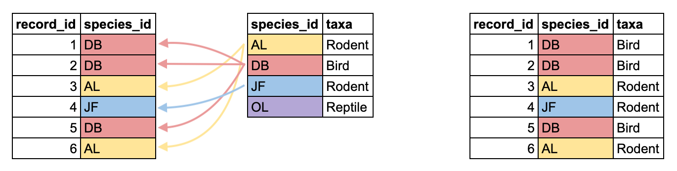
There are several types of joins in the dplyr package, which you can read more about here. We will use a function called left_join(), which takes two dataframes and adds the columns from the second dataframe to the first dataframe, matching rows based on the column name supplied to the by argument.
R
left_join(surveys_new, plots_new, by = "plot_id")
OUTPUT
# A tibble: 18,676 × 10
   record_id plot_id species_id sex   hindfoot_length weight  year month   day
       <dbl>   <dbl> <chr>      <chr>           <dbl>  <dbl> <dbl> <dbl> <int>
 1     16879       1 DM         F                  37     35  1990     1     6
 2     16880       1 OL         M                  21     28  1990     1     6
 3     16881       6 PF         M                  16      7  1990     1     6
 4     16882      23 RM         F                  17      9  1990     1     6
 5     16883      12 RM         M                  17     10  1990     1     6
 6     16884      24 RM         M                  17      9  1990     1     6
 7     16885      12 SF         M                  25     35  1990     1     6
 8     16886      24 SH         F                  30     73  1990     1     6
 9     16887      12 SF         M                  28     44  1990     1     6
10     16888      17 DO         M                  36     55  1990     1     6
# … with 18,666 more rows, and 1 more variable: plot_type <chr>
Now we have our surveys_new dataframe, still with 18676 rows, but now each row has a value for plot_type, corresponding to its entry in plot_id. We can assign this back to surveys_new, so that it now contains the information from both dataframes.
R
surveys_new <- left_join(surveys_new, plots_new, by = "plot_id")
We can repeat this process to get the information from species_new. surveys_new and species_new both have a species_id column, but we would like to add the genus, species, and taxa information to surveys_new.
R
surveys_new <- left_join(surveys_new, species_new, by = "species_id")

surveys_new
OUTPUT
# A tibble: 18,676 × 13
   record_id plot_id species_id sex   hindfoot_length weight  year month   day
       <dbl>   <dbl> <chr>      <chr>           <dbl>  <dbl> <dbl> <dbl> <int>
 1     16879       1 DM         F                  37     35  1990     1     6
 2     16880       1 OL         M                  21     28  1990     1     6
 3     16881       6 PF         M                  16      7  1990     1     6
 4     16882      23 RM         F                  17      9  1990     1     6
 5     16883      12 RM         M                  17     10  1990     1     6
 6     16884      24 RM         M                  17      9  1990     1     6
 7     16885      12 SF         M                  25     35  1990     1     6
 8     16886      24 SH         F                  30     73  1990     1     6
 9     16887      12 SF         M                  28     44  1990     1     6
10     16888      17 DO         M                  36     55  1990     1     6
# … with 18,666 more rows, and 4 more variables: plot_type <chr>, genus <chr>,
#   species <chr>, taxa <chr>
Now our surveys_new dataframe has all the information from our 3 files, and the same number of columns as our original surveys data.
Adding to the old data
Now that our old surveys data and surveys_new data are formatted in the same way, we can bind them together so we have data from all years in one data.frame. First let’s read our `surveys’ data back in.
R
surveys <- read_csv("data/cleaned/surveys_complete_77_89.csv")
OUTPUT
Rows: 16878 Columns: 13
── Column specification ────────────────────────────────────────────────────────
Delimiter: ","
chr (6): species_id, sex, genus, species, taxa, plot_type
dbl (7): record_id, month, day, year, plot_id, hindfoot_length, weight

ℹ Use `spec()` to retrieve the full column specification for this data.
ℹ Specify the column types or set `show_col_types = FALSE` to quiet this message.
Now we can use the bind_rows() function to bind the rows of our two data.frames together. The fact that our columns are not in the same order doesn’t matter, bind_rows() will detect thatt the column names are the same, and will rearrange them to match the first data.frame.
R
surveys_complete <- bind_rows(surveys, surveys_new)

surveys_complete
OUTPUT
# A tibble: 35,554 × 13
   record_id month   day  year plot_id species_id sex   hindfoot_length weight
       <dbl> <dbl> <dbl> <dbl>   <dbl> <chr>      <chr>           <dbl>  <dbl>
 1         1     7    16  1977       2 NL         M                  32     NA
 2         2     7    16  1977       3 NL         M                  33     NA
 3         3     7    16  1977       2 DM         F                  37     NA
 4         4     7    16  1977       7 DM         M                  36     NA
 5         5     7    16  1977       3 DM         M                  35     NA
 6         6     7    16  1977       1 PF         M                  14     NA
 7         7     7    16  1977       2 PE         F                  NA     NA
 8         8     7    16  1977       1 DM         M                  37     NA
 9         9     7    16  1977       1 DM         F                  34     NA
10        10     7    16  1977       6 PF         F                  20     NA
# … with 35,544 more rows, and 4 more variables: genus <chr>, species <chr>,
#   taxa <chr>, plot_type <chr>
We might be interested in indicating which rows of our data came from which source: the old data or the new. We can name the data.frames inside bind_rows(), and then give a new argument .id. This will give us a new column called source that contains a value of "old" for rows that came from surveys, and a value of "new" for rows that came from surveys_new.
R
surveys_complete <- bind_rows(old = surveys, new = surveys_new, .id = "source")

surveys_complete
OUTPUT
# A tibble: 35,554 × 14
   source record_id month   day  year plot_id species_id sex   hindfoot_length
   <chr>      <dbl> <dbl> <dbl> <dbl>   <dbl> <chr>      <chr>           <dbl>
 1 old            1     7    16  1977       2 NL         M                  32
 2 old            2     7    16  1977       3 NL         M                  33
 3 old            3     7    16  1977       2 DM         F                  37
 4 old            4     7    16  1977       7 DM         M                  36
 5 old            5     7    16  1977       3 DM         M                  35
 6 old            6     7    16  1977       1 PF         M                  14
 7 old            7     7    16  1977       2 PE         F                  NA
 8 old            8     7    16  1977       1 DM         M                  37
 9 old            9     7    16  1977       1 DM         F                  34
10 old           10     7    16  1977       6 PF         F                  20
# … with 35,544 more rows, and 5 more variables: weight <dbl>, genus <chr>,
#   species <chr>, taxa <chr>, plot_type <chr>
We have now successfully cleaned our new data and reshaped it to match our old data so they could be arranged into one data.frame covering all the years.
Back to ggplot2
position_dodge()-
coord_? patchwork-
label_wrap_gen()? theme_set()
R
surveys_complete %>%
count(year) %>%
ggplot(aes(x = year, y = n)) +
geom_line()
WARNING
Warning: Removed 1 row(s) containing missing values (geom_path).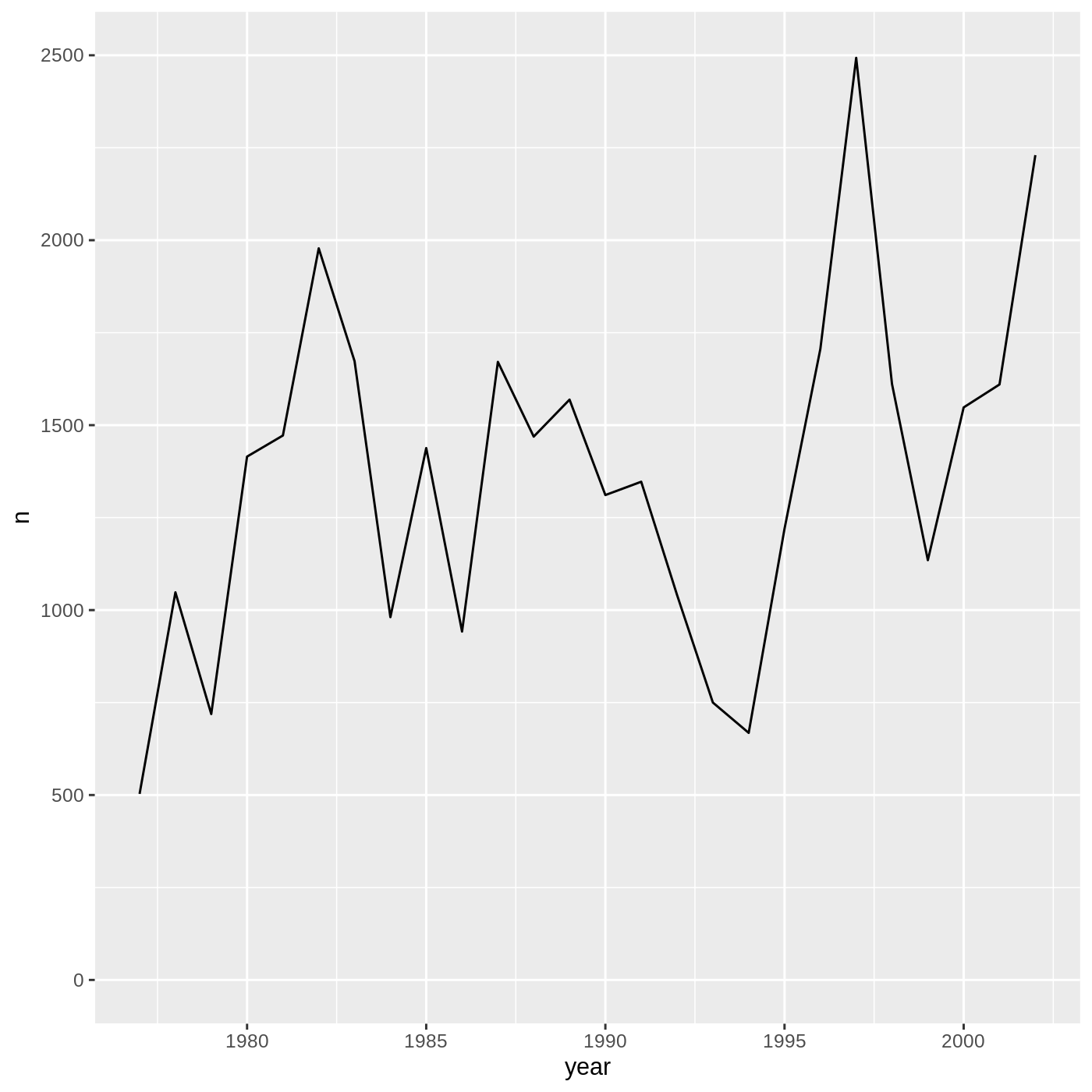
R
surveys_complete %>%
count(plot_type, sex) %>%
ggplot(aes(x = plot_type, y = n, fill = sex)) +
geom_col(position = position_dodge()) +
scale_x_discrete(labels = label_wrap_gen(10))
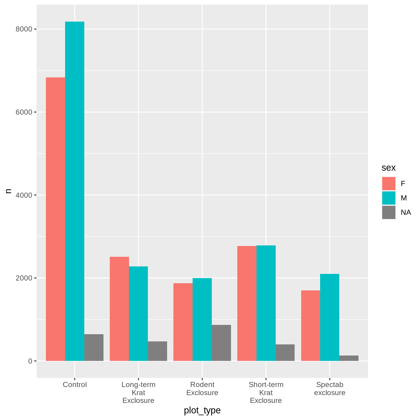
R
surveys_complete %>%
filter(!is.na(weight), !is.na(sex)) %>%
group_by(genus, year, sex) %>%
summarise(mean_weight = mean(weight)) %>%
ggplot(aes(x = year, y = mean_weight, color = genus)) +
geom_line() +
facet_wrap(vars(sex))
OUTPUT
`summarise()` has grouped output by 'genus', 'year'. You can override using the
`.groups` argument.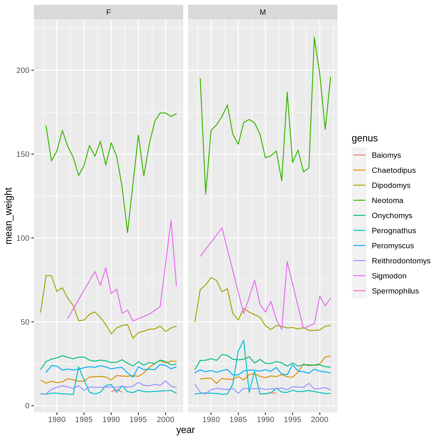
Setting limits with scale_ or xlim()/ylim() will remove data, so the slope of the line changes:
R
surveys_complete %>%
ggplot(aes(x = weight, y = hindfoot_length)) +
geom_point() +
geom_smooth(method = "lm") +
scale_x_continuous(limits = c(0,100))
OUTPUT
`geom_smooth()` using formula 'y ~ x'WARNING
Warning: Removed 7433 rows containing non-finite values (stat_smooth).WARNING
Warning: Removed 7433 rows containing missing values (geom_point).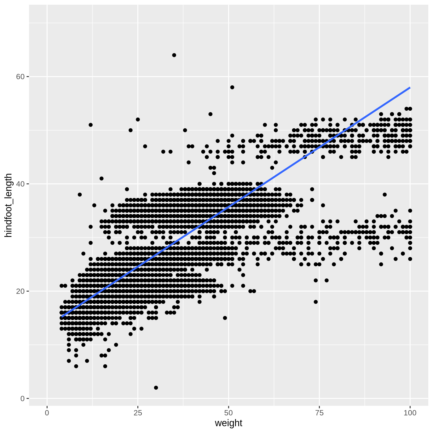
If you want to zoom in on the plot without removing data outside the limits, set the limits inside coord_cartestian():
R
surveys_complete %>%
ggplot(aes(x = weight, y = hindfoot_length)) +
geom_point() +
geom_smooth(method = "lm") +
coord_cartesian(xlim = c(0,100))
OUTPUT
`geom_smooth()` using formula 'y ~ x'WARNING
Warning: Removed 4812 rows containing non-finite values (stat_smooth).WARNING
Warning: Removed 4812 rows containing missing values (geom_point).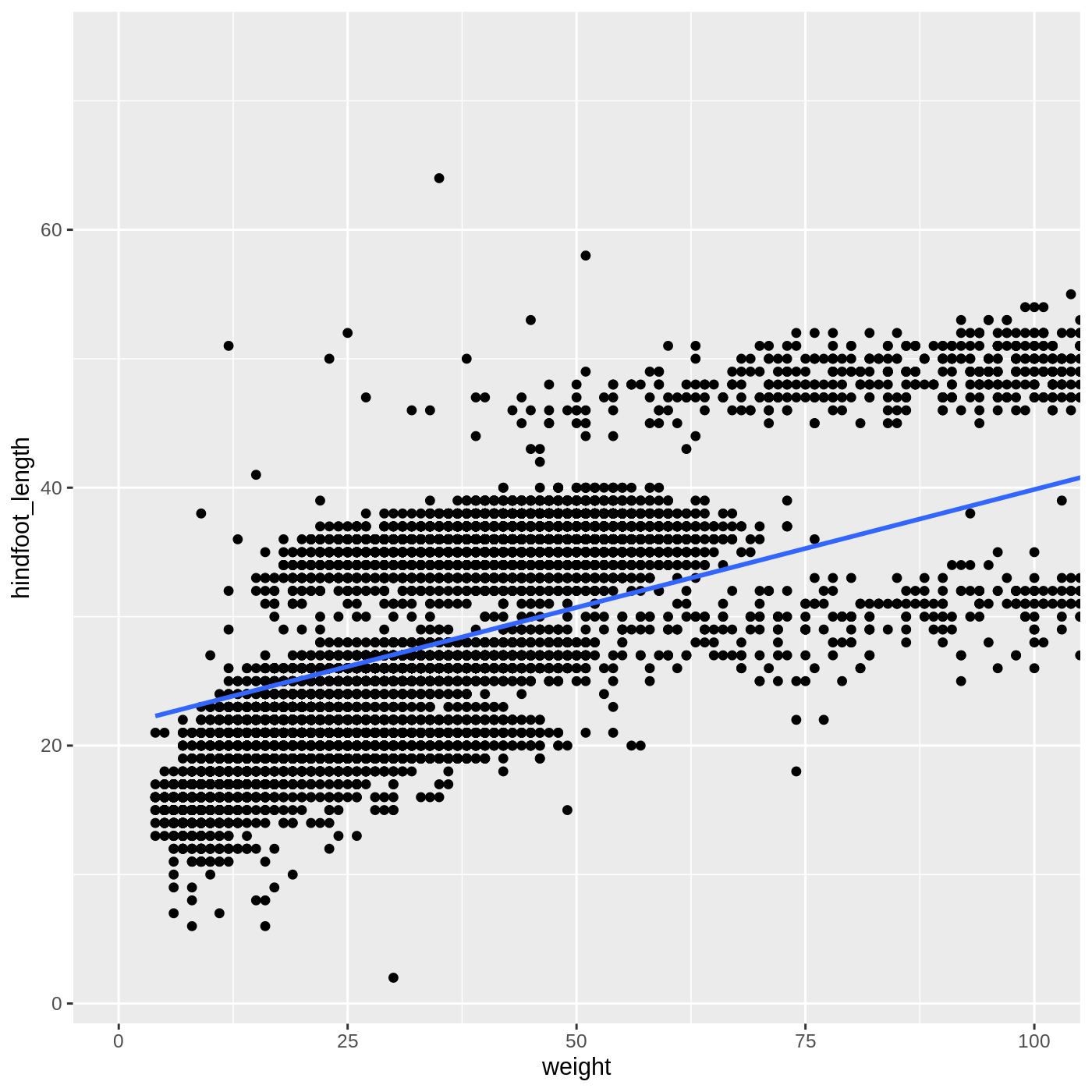
There are other coord_ functions if you need to plot using polar coordinates, map coordinates, or fix the aspect ratio of a plot.
Final outputs
Let’s go ahead and write our data to a CSV file so we can share it with others.
R
surveys_complete %>%
write_csv("data/cleaned/surveys_complete.csv")
Now we might be interested in looking at all of our data together. Try making some plots of your own to look at the whole dataset!
R
surveys_complete %>%
ggplot(aes(x = weight, y = hindfoot_length)) +
geom_point(alpha = 0.05) +
facet_wrap(vars(source))
WARNING
Warning: Removed 4812 rows containing missing values (geom_point).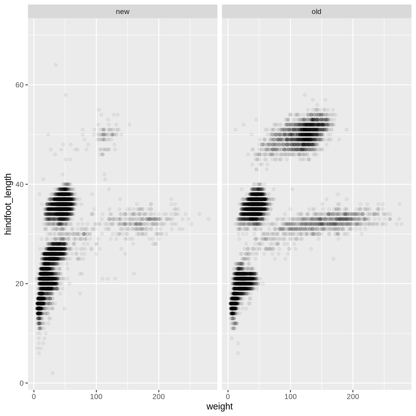
Keypoints
- it is always good to do preliminary investigations of new data
- there are often many ways to achieve the same goal, describing them with plain English or pseudocode can help you choose an approach
- the
read_delimited()function can read tabular data from multiple file formats - joins are powerful ways to combine multiple datasets
- it is a good idea to plan out the steps of your data cleaning and combining
Content from Extra Challenges
Last updated on 2022-11-29 | Edit this page
R
library(tidyverse)
surveys <- read_csv("data/cleaned/surveys_complete_77_89.csv")
Our points don’t actually turn out blue, because we defined the color inside of aes(). aes() is used for translating variables from the data into plot elements, like color. There is no variable in the data called “blue”.
Variable names inside aes() should not be wrapped in quotes.
When adding things like geom_ or scale_ functions to a ggplot(), you have to end a line with +, not begin a line with it.
When translating variables from the data, like weight and hindfoot_length, to elements of the plot, like x and y, you must put them inside aes().
species_id is a categorical variable, but scale_color_continuous() supplies a continuous color scale. scale_color_discrete() would give a discrete/categorical scale.