Multi-table joins
Learning objectives
- Focus on the third tidy data principle
- Each variable forms a column.
- Each observation forms a row.
- Each type of observational unit forms a table.
- Be able to use
dplyr’s join functions to merge tables
Joins
The third tidy data maxim states that each observation type gets its own table. The idea of multiple tables within a dataset will be familiar to anyone who has worked with a relational database but may seem foreign to those who have not.
The idea is this: Suppose we conduct a behavioral experiment that puts individuals in groups, and we measure both individual- and group-level variables. We should have a table for the individual-level variables and a separate table for the group-level variables. Then, should we need to merge them, we can do so using the join functions of dplyr.
The join functions are nicely illustrated in RStudio’s Data wrangling cheatsheet. Each function takes two data.frames and, optionally, the name(s) of columns on which to match. If no column names are provided, the functions match on all shared column names.
The different join functions control what happens to rows that exist in one table but not the other.
left_joinkeeps all the entries that are present in the left (first) table and excludes any that are only in the right table.right_joinkeeps all the entries that are present in the right table and excludes any that are only in the left table.inner_joinkeeps only the entries that are present in both tables.inner_joinis the only function that guarantees you won’t generate any missing entries.full_joinkeeps all of the entries in both tables, regardless of whether or not they appear in the other table.
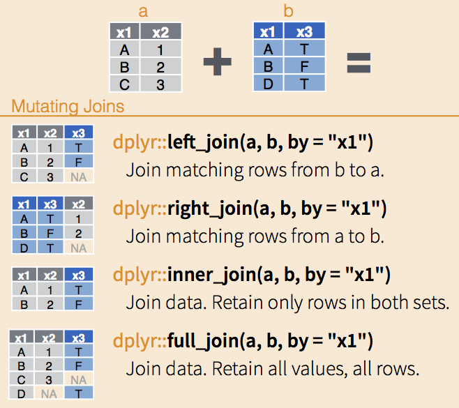
dplyr joins, via RStudio
Practice with joins
Fabricate some example data
set.seed(12345)
x <- data.frame(key= LETTERS[c(1:3, 5)],
                value1 = sample(1:10, 4),
                stringsAsFactors = FALSE)
y <- data.frame(key= LETTERS[c(1:4)],
                value2 = sample(1:10, 4),
                stringsAsFactors = FALSE)

x
## key value1
## 1 A 3
## 2 B 8
## 3 C 2
## 4 E 5y## key value2
## 1 A 8
## 2 B 2
## 3 C 6
## 4 D 3“Joining” joins
# What's in both x and y?
inner_join(x, y, by = "key")
## key value1 value2
## 1 A 3 8
## 2 B 8 2
## 3 C 2 6# What's in X and bring with it the stuff that matches in Y
left_join(x, y, by = "key")## key value1 value2
## 1 A 3 8
## 2 B 8 2
## 3 C 2 6
## 4 E 5 NA# What's in Y and bring with it the stuff that matches in Y
right_join(x, y, by = "key")## key value1 value2
## 1 A 3 8
## 2 B 8 2
## 3 C 2 6
## 4 D NA 3# Give me everything!
full_join(x, y, by = "key")## key value1 value2
## 1 A 3 8
## 2 B 8 2
## 3 C 2 6
## 4 E 5 NA
## 5 D NA 3Filtering “joins”
# Give me the stuff in X that is also in Y
semi_join(x, y, by = "key")
## key value1
## 1 A 3
## 2 B 8
## 3 C 2# Give me the stuff in X that is not in Y
anti_join(x, y, by = "key")## key value1
## 1 E 5# Want everything that doesn't match?
full_join(anti_join(x,y, by = "key"), anti_join(y,x, by = "key"), by= "key")## key value1 value2
## 1 E 5 NA
## 2 D NA 3# keys with different names?
x <- data.frame(keyX = LETTERS[c(1:3, 5)],
value1 = sample(1:10, 4),
stringsAsFactors = FALSE)
y <- data.frame(keyY = LETTERS[c(1:4)],
value2 = sample(1:10, 4),
stringsAsFactors = FALSE)
x## keyX value1
## 1 A 6
## 2 B 7
## 3 C 10
## 4 E 2y## keyY value2
## 1 A 1
## 2 B 8
## 3 C 7
## 4 D 6full_join(x, y) #should error out## Error: `by` required, because the data sources have no common variablesfull_join(x, y, by=c("keyX" = "keyY"))## keyX value1 value2
## 1 A 6 1
## 2 B 7 8
## 3 C 10 7
## 4 E 2 NA
## 5 D NA 6Set Operations
df1 <- data_frame(x = LETTERS[1:2],
                  y = c(1L, 1L))
## Warning: `data_frame()` is deprecated, use `tibble()`.
## This warning is displayed once per session.df2 <- data_frame(x = LETTERS[1:2],
y = 1:2)
df1## # A tibble: 2 x 2
## x y
## <chr> <int>
## 1 A 1
## 2 B 1df2## # A tibble: 2 x 2
## x y
## <chr> <int>
## 1 A 1
## 2 B 2# Which rows are common in both datasets?
dplyr::intersect(df1, df2)## # A tibble: 1 x 2
## x y
## <chr> <int>
## 1 A 1#Want all unique rows between both datasets?
dplyr::union(df1, df2)## # A tibble: 3 x 2
## x y
## <chr> <int>
## 1 A 1
## 2 B 1
## 3 B 2#What's unique to df1?
dplyr::setdiff(df1, df2)## # A tibble: 1 x 2
## x y
## <chr> <int>
## 1 B 1#What's unique to df2?
dplyr::setdiff(df2, df1)## # A tibble: 1 x 2
## x y
## <chr> <int>
## 1 B 2Practice with joins using gapminder
We will practice on our continents data.frame from module 2 and the gapminder data.frame. Note how these are tidy data: We have observations at the level of continent and at the level of country, so they go in different tables. The continent column in the gapminder data.frame allows us to link them now. If continents data.frame isn’t in your Environment, load it and recall what it consists of:
load('data/continents.RDA')
continents
## continent area_km2 population percent_total_pop
## 1 Africa 30370000 1022234000 15.0
## 2 Americas 42330000 934611000 14.0
## 3 Antarctica 13720000 4490 0.0
## 4 Asia 43820000 4164252000 60.0
## 5 Europe 10180000 738199000 11.0
## 6 Oceania 9008500 29127000 0.4We can join the two data.frames using any of the dplyr functions. We will pass the results to str to avoid printing more than we can read, and to get more high-level information on the resulting data.frames.
left_join(gapminder, continents) ## Joining, by = "continent"## Warning: Column `continent` joining factor and character vector, coercing
## into character vector## # A tibble: 1,704 x 9
## country continent year lifeExp pop gdpPercap area_km2 population
## <fct> <chr> <int> <dbl> <int> <dbl> <dbl> <dbl>
## 1 Afghan… Asia 1952 28.8 8.43e6 779. 43820000 4164252000
## 2 Afghan… Asia 1957 30.3 9.24e6 821. 43820000 4164252000
## 3 Afghan… Asia 1962 32.0 1.03e7 853. 43820000 4164252000
## 4 Afghan… Asia 1967 34.0 1.15e7 836. 43820000 4164252000
## 5 Afghan… Asia 1972 36.1 1.31e7 740. 43820000 4164252000
## 6 Afghan… Asia 1977 38.4 1.49e7 786. 43820000 4164252000
## 7 Afghan… Asia 1982 39.9 1.29e7 978. 43820000 4164252000
## 8 Afghan… Asia 1987 40.8 1.39e7 852. 43820000 4164252000
## 9 Afghan… Asia 1992 41.7 1.63e7 649. 43820000 4164252000
## 10 Afghan… Asia 1997 41.8 2.22e7 635. 43820000 4164252000
## # … with 1,694 more rows, and 1 more variable: percent_total_pop <dbl>right_join(gapminder, continents)## Joining, by = "continent"## Warning: Column `continent` joining factor and character vector, coercing
## into character vector## # A tibble: 1,705 x 9
## country continent year lifeExp pop gdpPercap area_km2 population
## <fct> <chr> <int> <dbl> <int> <dbl> <dbl> <dbl>
## 1 Algeria Africa 1952 43.1 9.28e6 2449. 30370000 1022234000
## 2 Algeria Africa 1957 45.7 1.03e7 3014. 30370000 1022234000
## 3 Algeria Africa 1962 48.3 1.10e7 2551. 30370000 1022234000
## 4 Algeria Africa 1967 51.4 1.28e7 3247. 30370000 1022234000
## 5 Algeria Africa 1972 54.5 1.48e7 4183. 30370000 1022234000
## 6 Algeria Africa 1977 58.0 1.72e7 4910. 30370000 1022234000
## 7 Algeria Africa 1982 61.4 2.00e7 5745. 30370000 1022234000
## 8 Algeria Africa 1987 65.8 2.33e7 5681. 30370000 1022234000
## 9 Algeria Africa 1992 67.7 2.63e7 5023. 30370000 1022234000
## 10 Algeria Africa 1997 69.2 2.91e7 4797. 30370000 1022234000
## # … with 1,695 more rows, and 1 more variable: percent_total_pop <dbl>These operations produce slightly different results, either 1704 or 1705 observations. Can you figure out why? Antarctica contains no countries so doesn’t appear in the gapminder data.frame. When we use left_join it gets filtered from the results, but when we use right_join it appears, with missing values for all of the country-level variables:
right_join(gapminder, continents) %>%
  filter(continent == "Antarctica")
## Joining, by = "continent"## Warning: Column `continent` joining factor and character vector, coercing
## into character vector## # A tibble: 1 x 9
## country continent year lifeExp pop gdpPercap area_km2 population
## <fct> <chr> <int> <dbl> <int> <dbl> <dbl> <dbl>
## 1 <NA> Antarcti… NA NA NA NA 13720000 4490
## # … with 1 more variable: percent_total_pop <dbl>There’s another problem in this data.frame – it has two population measures, one by continent and one by country and it’s not clear which is which! Let’s rename a couple of columns.
right_join(gapminder, continents) %>%
  rename(country_pop = pop, continent_pop = population)
## Joining, by = "continent"## Warning: Column `continent` joining factor and character vector, coercing
## into character vector## # A tibble: 1,705 x 9
## country continent year lifeExp country_pop gdpPercap area_km2
## <fct> <chr> <int> <dbl> <int> <dbl> <dbl>
## 1 Algeria Africa 1952 43.1 9279525 2449. 30370000
## 2 Algeria Africa 1957 45.7 10270856 3014. 30370000
## 3 Algeria Africa 1962 48.3 11000948 2551. 30370000
## 4 Algeria Africa 1967 51.4 12760499 3247. 30370000
## 5 Algeria Africa 1972 54.5 14760787 4183. 30370000
## 6 Algeria Africa 1977 58.0 17152804 4910. 30370000
## 7 Algeria Africa 1982 61.4 20033753 5745. 30370000
## 8 Algeria Africa 1987 65.8 23254956 5681. 30370000
## 9 Algeria Africa 1992 67.7 26298373 5023. 30370000
## 10 Algeria Africa 1997 69.2 29072015 4797. 30370000
## # … with 1,695 more rows, and 2 more variables: continent_pop <dbl>,
## # percent_total_pop <dbl>Challenge – Putting the pieces together
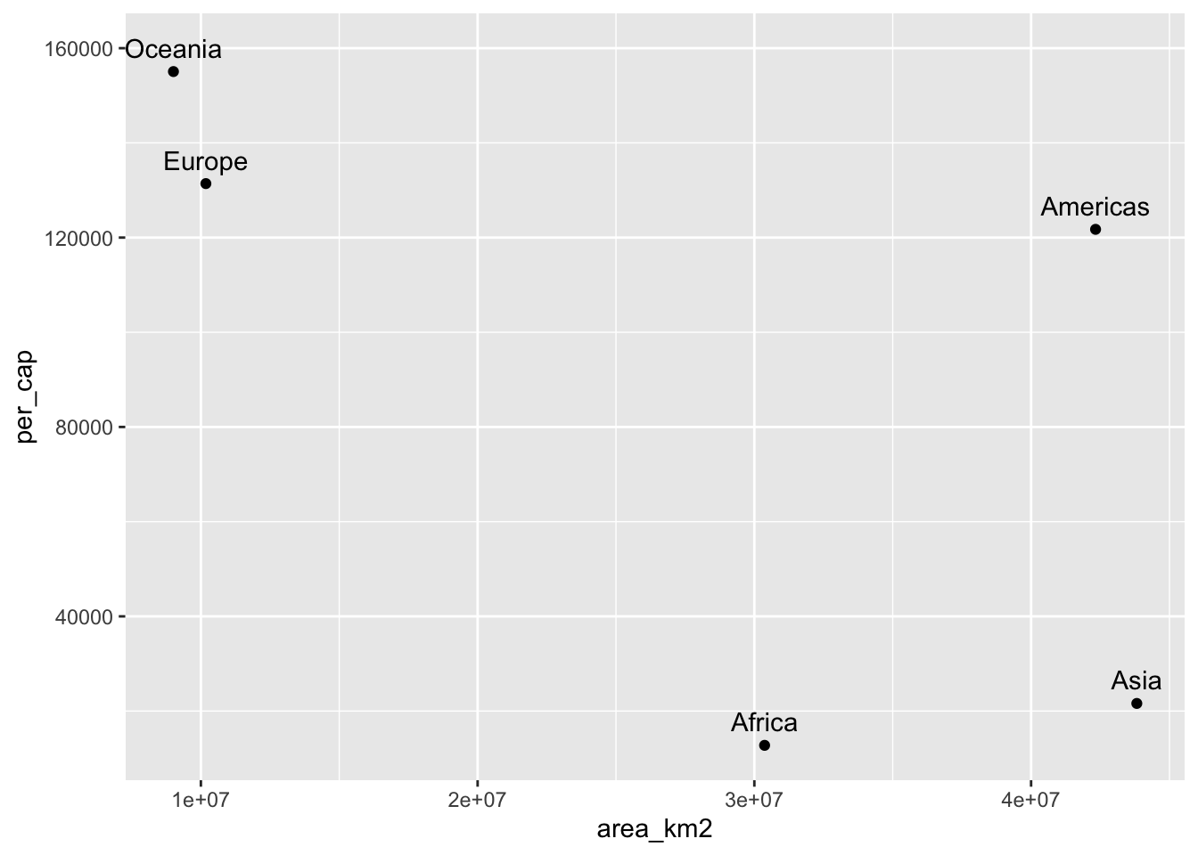
A colleague suggests that the more land area an individual has, the greater their gdp will be and that this relationship will be observable at any scale of observation. You chuckle and mutter “Not at the continental scale,” but your colleague insists. Test your colleague’s hypothesis by:
- Calculating the total GDP of each continent, - Hint: Use
dplyr’sgroup_byandsummarize- Joining the resulting data.frame to the
continentsdata.frame,- Calculating the per-capita GDP for each continent, and
- Plotting per-capita gdp versus population density.
Challenge solutions
Solution to Challenge – Putting the pieces together
library(ggplot2)

gapminder %>%
  mutate(GDP = gdpPercap * pop) %>%  # Calculate country-level GDP
  group_by(continent) %>%  # Group by continent
  summarize(cont_gdp = sum(GDP)) %>%  # Calculate continent-level GDP
# Join the continent-GDP data.frame to the continents data.frame
    left_join(continents) %>%
# Calculate continent-level per-capita GDP
    mutate(per_cap = cont_gdp / population) %>%
# Plot gdp versus land area
    ggplot(aes(x = area_km2, y = per_cap)) +
# Draw points
    geom_point() +
# And label them
    geom_text(aes(label = continent), nudge_y = 5e3)
## Joining, by = "continent"## Warning: Column `continent` joining factor and character vector, coercing ## into character vector
Practice with joins using surveys
To illustrate how to use dplyr with these complex queries, we are going to join the plots and surveys tables. The plots table in the database contains information about the different plots surveyed by the researchers.
The datasets can be found here: plots.csv, surveys.csv, and species.csv.
Download them and save them to your downloads folder. Alternatively, copy the link and use the read_csv() function directly on that.
plots <- read_csv("data/plots.csv")## Parsed with column specification:
## cols(
## plot_id = col_double(),
## plot_type = col_character()
## )plots## # A tibble: 24 x 2
## plot_id plot_type
## <dbl> <chr>
## 1 1 Spectab exclosure
## 2 2 Control
## 3 3 Long-term Krat Exclosure
## 4 4 Control
## 5 5 Rodent Exclosure
## 6 6 Short-term Krat Exclosure
## 7 7 Rodent Exclosure
## 8 8 Control
## 9 9 Spectab exclosure
## 10 10 Rodent Exclosure
## # … with 14 more rowsThe plot_id column also features in the surveys table:
surveys <- read_csv("data/surveys.csv")## Parsed with column specification:
## cols(
## record_id = col_double(),
## month = col_double(),
## day = col_double(),
## year = col_double(),
## plot_id = col_double(),
## species_id = col_character(),
## sex = col_character(),
## hindfoot_length = col_double(),
## weight = col_double()
## )surveys## # A tibble: 35,549 x 9
## record_id month day year plot_id species_id sex hindfoot_length
## <dbl> <dbl> <dbl> <dbl> <dbl> <chr> <chr> <dbl>
## 1 1 7 16 1977 2 NL M 32
## 2 2 7 16 1977 3 NL M 33
## 3 3 7 16 1977 2 DM F 37
## 4 4 7 16 1977 7 DM M 36
## 5 5 7 16 1977 3 DM M 35
## 6 6 7 16 1977 1 PF M 14
## 7 7 7 16 1977 2 PE F NA
## 8 8 7 16 1977 1 DM M 37
## 9 9 7 16 1977 1 DM F 34
## 10 10 7 16 1977 6 PF F 20
## # … with 35,539 more rows, and 1 more variable: weight <dbl>Because plot_id is listed in both tables, we can use it to look up matching records, and join the two tables.

diagram illustrating inner and left joins
For example, to extract all surveys for the first plot, which has plot_id 1, we can do:
plots %>%
  filter(plot_id == 1) %>%
  inner_join(surveys)
## Joining, by = "plot_id"## # A tibble: 1,995 x 10
## plot_id plot_type record_id month day year species_id sex
## <dbl> <chr> <dbl> <dbl> <dbl> <dbl> <chr> <chr>
## 1 1 Spectab … 6 7 16 1977 PF M
## 2 1 Spectab … 8 7 16 1977 DM M
## 3 1 Spectab … 9 7 16 1977 DM F
## 4 1 Spectab … 78 8 19 1977 PF M
## 5 1 Spectab … 80 8 19 1977 DS M
## 6 1 Spectab … 218 9 13 1977 PF M
## 7 1 Spectab … 222 9 13 1977 DS M
## 8 1 Spectab … 239 9 13 1977 DS M
## 9 1 Spectab … 263 10 16 1977 DM M
## 10 1 Spectab … 270 10 16 1977 DM F
## # … with 1,985 more rows, and 2 more variables: hindfoot_length <dbl>,
## # weight <dbl>Challenge
Write some code that returns the number of rodents observed in each plot in each year. Start by reading in the species dataframe.
species <- read_csv("data/species.csv")## Parsed with column specification: ## cols( ## species_id = col_character(), ## genus = col_character(), ## species = col_character(), ## taxa = col_character() ## )Hint: All the information you need isn’t contained in one single dataframe just yet. The “taxa” information is contained in the species dataframe, and the observation data is contained in the surveys dataframe. Write some code that joins the species and survey tables together on a common column. What are the common columns?
Hint: How would you use a split-apply-combine strategy to count the number of observations per plot, per year? Which part of this hint refers to the “splitting”, and which part refers to the “applying”?
Hint: How would you subset the resulting dataframe to just include the rodents?
glimpse(surveys)## Observations: 35,549 ## Variables: 9 ## $ record_id <dbl> 1, 2, 3, 4, 5, 6, 7, 8, 9, 10, 11, 12, 13, 14, 1… ## $ month <dbl> 7, 7, 7, 7, 7, 7, 7, 7, 7, 7, 7, 7, 7, 7, 7, 7, … ## $ day <dbl> 16, 16, 16, 16, 16, 16, 16, 16, 16, 16, 16, 16, … ## $ year <dbl> 1977, 1977, 1977, 1977, 1977, 1977, 1977, 1977, … ## $ plot_id <dbl> 2, 3, 2, 7, 3, 1, 2, 1, 1, 6, 5, 7, 3, 8, 6, 4, … ## $ species_id <chr> "NL", "NL", "DM", "DM", "DM", "PF", "PE", "DM", … ## $ sex <chr> "M", "M", "F", "M", "M", "M", "F", "M", "F", "F"… ## $ hindfoot_length <dbl> 32, 33, 37, 36, 35, 14, NA, 37, 34, 20, 53, 38, … ## $ weight <dbl> NA, NA, NA, NA, NA, NA, NA, NA, NA, NA, NA, NA, …glimpse(species)## Observations: 54 ## Variables: 4 ## $ species_id <chr> "AB", "AH", "AS", "BA", "CB", "CM", "CQ", "CS", "CT",… ## $ genus <chr> "Amphispiza", "Ammospermophilus", "Ammodramus", "Baio… ## $ species <chr> "bilineata", "harrisi", "savannarum", "taylori", "bru… ## $ taxa <chr> "Bird", "Rodent", "Bird", "Rodent", "Bird", "Bird", "…## with dplyr syntax surveys %>% left_join(species) %>% group_by(plot_id, taxa, year) %>% summarize(n = n()) %>% filter(taxa == "Rodent")## Joining, by = "species_id"## # A tibble: 619 x 4 ## # Groups: plot_id, taxa [24] ## plot_id taxa year n ## <dbl> <chr> <dbl> <int> ## 1 1 Rodent 1977 22 ## 2 1 Rodent 1978 57 ## 3 1 Rodent 1979 26 ## 4 1 Rodent 1980 75 ## 5 1 Rodent 1981 79 ## 6 1 Rodent 1982 109 ## 7 1 Rodent 1983 129 ## 8 1 Rodent 1984 49 ## 9 1 Rodent 1985 102 ## 10 1 Rodent 1986 57 ## # … with 609 more rows# Alternatively, filter to rodents *before* summarizing by plot and year surveys %>% left_join(species) %>% filter(taxa == "Rodent") %>% group_by(plot_id, year) %>% summarize(n = n())## Joining, by = "species_id"## # A tibble: 619 x 3 ## # Groups: plot_id [24] ## plot_id year n ## <dbl> <dbl> <int> ## 1 1 1977 22 ## 2 1 1978 57 ## 3 1 1979 26 ## 4 1 1980 75 ## 5 1 1981 79 ## 6 1 1982 109 ## 7 1 1983 129 ## 8 1 1984 49 ## 9 1 1985 102 ## 10 1 1986 57 ## # … with 609 more rows
Challenge
Write some code that returns the total number of rodents in each genus caught in the different plot types.
Hint: Not all the data you need are contained in 1 dataframe. The plot_type data are in the plots dataframe, the taxa data are in the species dataframe, and the observation data are in the surveys dataframe. Start by joining these three dataframes together.
Hint: Think “split-apply-combine”. We want to count the number of observations in each group defined by
plot_typeandgenuscombinations. That is, what is the count of observations per plot_type, per genus for just the Rodent taxa.genus_counts <- surveys %>% left_join(plots) %>% left_join(species) %>% filter(taxa == "Rodent") %>% group_by(plot_type, genus, taxa) %>% summarize(n = n())## Joining, by = "plot_id"Joining, by = "species_id"genus_counts## # A tibble: 59 x 4 ## # Groups: plot_type, genus [59] ## plot_type genus taxa n ## <chr> <chr> <chr> <int> ## 1 Control Ammospermophilus Rodent 125 ## 2 Control Baiomys Rodent 1 ## 3 Control Chaetodipus Rodent 1902 ## 4 Control Dipodomys Rodent 9847 ## 5 Control Neotoma Rodent 610 ## 6 Control Onychomys Rodent 1481 ## 7 Control Perognathus Rodent 435 ## 8 Control Peromyscus Rodent 464 ## 9 Control Reithrodontomys Rodent 415 ## 10 Control Rodent Rodent 5 ## # … with 49 more rows
This lesson is adapted from the Software Carpentry: R for Reproducible Scientific Analysis Multi-Table Joins materials, Brandon Hurr’s dplyr II: Joins and Set Ops presentation to the Davis R UsersGroup on Februrary 2, 2016, and the Data Carpentry: R for Data Analysis and Visualization of Ecological Data R and Databases materials.