Manipulating and analyzing data with dplyr; Exporting data
Learning Objectives
- Describe the purpose of the
dplyrandtidyrpackages. - Select certain columns in a data frame with the
dplyrfunctionselect. - Select certain rows in a data frame according to filtering conditions with the
dplyrfunctionfilter. - Link the output of one
dplyrfunction to the input of another function with the ‘pipe’ operator%>%. - Add new columns to a data frame that are functions of existing columns with
mutate. - Use the split-apply-combine concept for data analysis.
- Use
summarize,group_by, andtallyto split a data frame into groups of observations, apply a summary statistics for each group, and then combine the results. - Use
joinfunctions to join two dataframes together - Describe the concept of a wide and a long table format and for which purpose those formats are useful.
- Reshape a data frame from long to wide format and back with the
pivot_widerandpivot_longercommands from thetidyrpackage.
Data Manipulation using dplyr and tidyr
Bracket subsetting is handy, but it can be cumbersome and difficult to read, especially for complicated operations. Enter dplyr. dplyr is a package for making tabular data manipulation easier. It pairs nicely with tidyr which enables you to swiftly convert between different data formats for plotting and analysis.
Packages in R are basically sets of additional functions that let you do more stuff. The functions we’ve been using so far, like str() or data.frame(), come built into R; packages give you access to more of them. Before you use a package for the first time you need to install it on your machine, and then you should import it in every subsequent R session when you need it. You should already have installed the tidyverse package. This is an “umbrella-package” that installs several packages useful for data analysis which work together well such as tidyr, dplyr, ggplot2, tibble, etc.
The tidyverse package tries to address 3 major problems with some of base R functions: 1. The results from a base R function sometimes depend on the type of data. 2. Using R expressions in a non standard way, which can be confusing for new learners. 3. Hidden arguments, having default operations that new learners are not aware of.
To load the package type:
library("tidyverse") ## load the tidyverse packages, incl. dplyrWhat are dplyr and tidyr?
The package dplyr provides easy tools for the most common data manipulation tasks. It is built to work directly with data frames, with many common tasks optimized by being written in a compiled language (C++). An additional feature is the ability to work directly with data stored in an external database. The benefits of doing this are that the data can be managed natively in a relational database, queries can be conducted on that database, and only the results of the query are returned.
This addresses a common problem with R in that all operations are conducted in-memory and thus the amount of data you can work with is limited by available memory. The database connections essentially remove that limitation in that you can connect to a database of many hundreds of GB, conduct queries on it directly, and pull back into R only what you need for analysis.
The package tidyr addresses the common problem of wanting to reshape your data for plotting and use by different R functions. Sometimes we want data sets where we have one row per measurement. Sometimes we want a data frame where each measurement type has its own column, and rows are instead more aggregated groups - like plots or aquaria. Moving back and forth between these formats is nontrivial, and tidyr gives you tools for this and more sophisticated data manipulation.
To learn more about dplyr and tidyr after the workshop, you may want to check out this handy data transformation with dplyr cheatsheet and this one about tidyr.
We’ll read in our data using the read_csv() function, from the tidyverse package readr, instead of read.csv(), the base function for reading in data. The data we are going to be using today should already be in your R_DAVIS_2020 project in the folder data.
surveys <- read_csv("data/portal_data_joined.csv")## Parsed with column specification:
## cols(
## record_id = col_double(),
## month = col_double(),
## day = col_double(),
## year = col_double(),
## plot_id = col_double(),
## species_id = col_character(),
## sex = col_character(),
## hindfoot_length = col_double(),
## weight = col_double(),
## genus = col_character(),
## species = col_character(),
## taxa = col_character(),
## plot_type = col_character()
## )## inspect the data
str(surveys)Notice that the class of the data is now tbl_df This is referred to as a “tibble”. Tibbles are almost identical to R’s standard data frames, but they tweak some of the old behaviors of data frames. For our purposes the only differences between data frames and tibbles are that:
- When you print a tibble, R displays the data type of each column under its name; it prints only the first few rows of data and only as many columns as fit on one screen.
- Columns of class
characterare never automatically converted into factors.
Selecting columns and filtering rows
We’re going to learn some of the most common dplyr functions: select(), filter(), mutate(), group_by(), summarize(), and join. To select columns of a data frame, use select(). The first argument to this function is the data frame (surveys), and the subsequent arguments are the columns to keep.
select(surveys, plot_id, species_id, weight)To choose rows based on a specific criteria, use filter():
filter(surveys, year == 1995)## # A tibble: 1,180 x 13
## record_id month day year plot_id species_id sex hindfoot_length
## <dbl> <dbl> <dbl> <dbl> <dbl> <chr> <chr> <dbl>
## 1 22314 6 7 1995 2 NL M 34
## 2 22728 9 23 1995 2 NL F 32
## 3 22899 10 28 1995 2 NL F 32
## 4 23032 12 2 1995 2 NL F 33
## 5 22003 1 11 1995 2 DM M 37
## 6 22042 2 4 1995 2 DM F 36
## 7 22044 2 4 1995 2 DM M 37
## 8 22105 3 4 1995 2 DM F 37
## 9 22109 3 4 1995 2 DM M 37
## 10 22168 4 1 1995 2 DM M 36
## # … with 1,170 more rows, and 5 more variables: weight <dbl>, genus <chr>,
## # species <chr>, taxa <chr>, plot_type <chr>select is used for rows and filter is used for columns.
Pipes
What if you want to select and filter at the same time? There are three ways to do this: use intermediate steps, nested functions, or pipes.
With intermediate steps, you create a temporary data frame and use that as input to the next function, like this:
surveys2 <- filter(surveys, weight < 5)
surveys_sml <- select(surveys2, species_id, sex, weight)
This is readable, but can clutter up your workspace with lots of objects that you have to name individually. With multiple steps, that can be hard to keep track of.
You can also nest functions (i.e. one function inside of another), like this:
surveys_sml <- select(filter(surveys, weight < 5), species_id, sex, weight)This is handy, but can be difficult to read if too many functions are nested, as R evaluates the expression from the inside out (in this case, filtering, then selecting).
The last option is pipes. Pipes let you take the output of one function and send it directly to the next, which is useful when you need to do many things to the same dataset. Pipes in R look like %>% and are made available via the magrittr package, installed automatically with dplyr. If you use RStudio, you can type the pipe with Ctrl + Shift + M if you have a PC or Cmd + Shift + M if you have a Mac.
surveys %>%
  filter(weight < 5) %>%
  select(species_id, sex, weight)
## # A tibble: 17 x 3
## species_id sex weight
## <chr> <chr> <dbl>
## 1 PF F 4
## 2 PF F 4
## 3 PF M 4
## 4 RM F 4
## 5 RM M 4
## 6 PF <NA> 4
## 7 PP M 4
## 8 RM M 4
## 9 RM M 4
## 10 RM M 4
## 11 PF M 4
## 12 PF F 4
## 13 RM M 4
## 14 RM M 4
## 15 RM F 4
## 16 RM M 4
## 17 RM M 4In the above code, we use the pipe to send the surveys dataset first through filter() to keep rows where weight is less than 5, then through select() to keep only the species_id, sex, and weight columns. Since %>% takes the object on its left and passes it as the first argument to the function on its right, we don’t need to explicitly include the data frame as an argument to the filter() and select() functions any more.
Some may find it helpful to read the pipe like the word “then”. For instance, in the above example, we took the data frame surveys, then we filtered for rows with weight < 5, then we selected columns species_id, sex, and weight. The dplyr functions by themselves are somewhat simple, but by combining them into linear workflows with the pipe, we can accomplish more complex manipulations of data frames.
If we want to create a new object with this smaller version of the data, we can assign it a new name:
surveys_sml <- surveys %>%
  filter(weight < 5) %>%
  select(species_id, sex, weight)

surveys_sml
## # A tibble: 17 x 3
## species_id sex weight
## <chr> <chr> <dbl>
## 1 PF F 4
## 2 PF F 4
## 3 PF M 4
## 4 RM F 4
## 5 RM M 4
## 6 PF <NA> 4
## 7 PP M 4
## 8 RM M 4
## 9 RM M 4
## 10 RM M 4
## 11 PF M 4
## 12 PF F 4
## 13 RM M 4
## 14 RM M 4
## 15 RM F 4
## 16 RM M 4
## 17 RM M 4Note that the final data frame is the leftmost part of this expression.
Challenge
Using pipes, subset the surveys data to include individuals collected before 1995 and retain only the columns year, sex, and weight. Name this dataframe surveys_challenge
ANSWER
surveys_challenge <- surveys %>%
    filter(year < 1995) %>%
    select(year, sex, weight)
Mutate
Frequently you’ll want to create new columns based on the values in existing columns, for example to do unit conversions, or to find the ratio of values in two columns. For this we’ll use mutate().
To create a new column of weight in kg:
surveys %>%
  mutate(weight_kg = weight / 1000)
## # A tibble: 34,786 x 14
## record_id month day year plot_id species_id sex hindfoot_length
## <dbl> <dbl> <dbl> <dbl> <dbl> <chr> <chr> <dbl>
## 1 1 7 16 1977 2 NL M 32
## 2 72 8 19 1977 2 NL M 31
## 3 224 9 13 1977 2 NL <NA> NA
## 4 266 10 16 1977 2 NL <NA> NA
## 5 349 11 12 1977 2 NL <NA> NA
## 6 363 11 12 1977 2 NL <NA> NA
## 7 435 12 10 1977 2 NL <NA> NA
## 8 506 1 8 1978 2 NL <NA> NA
## 9 588 2 18 1978 2 NL M NA
## 10 661 3 11 1978 2 NL <NA> NA
## # … with 34,776 more rows, and 6 more variables: weight <dbl>,
## # genus <chr>, species <chr>, taxa <chr>, plot_type <chr>,
## # weight_kg <dbl>You can also create a second new column based on the first new column within the same call of mutate():
surveys %>%
  mutate(weight_kg = weight / 1000,
         weight_kg2 = weight_kg * 2)
## # A tibble: 34,786 x 15
## record_id month day year plot_id species_id sex hindfoot_length
## <dbl> <dbl> <dbl> <dbl> <dbl> <chr> <chr> <dbl>
## 1 1 7 16 1977 2 NL M 32
## 2 72 8 19 1977 2 NL M 31
## 3 224 9 13 1977 2 NL <NA> NA
## 4 266 10 16 1977 2 NL <NA> NA
## 5 349 11 12 1977 2 NL <NA> NA
## 6 363 11 12 1977 2 NL <NA> NA
## 7 435 12 10 1977 2 NL <NA> NA
## 8 506 1 8 1978 2 NL <NA> NA
## 9 588 2 18 1978 2 NL M NA
## 10 661 3 11 1978 2 NL <NA> NA
## # … with 34,776 more rows, and 7 more variables: weight <dbl>,
## # genus <chr>, species <chr>, taxa <chr>, plot_type <chr>,
## # weight_kg <dbl>, weight_kg2 <dbl>If this runs off your screen and you just want to see the first few rows, you can use a pipe to view the head() of the data. (Pipes work with non-dplyr functions, too, as long as the dplyr or magrittr package is loaded).
surveys %>%
  mutate(weight_kg = weight / 1000) %>%
  head()
## # A tibble: 6 x 14
## record_id month day year plot_id species_id sex hindfoot_length
## <dbl> <dbl> <dbl> <dbl> <dbl> <chr> <chr> <dbl>
## 1 1 7 16 1977 2 NL M 32
## 2 72 8 19 1977 2 NL M 31
## 3 224 9 13 1977 2 NL <NA> NA
## 4 266 10 16 1977 2 NL <NA> NA
## 5 349 11 12 1977 2 NL <NA> NA
## 6 363 11 12 1977 2 NL <NA> NA
## # … with 6 more variables: weight <dbl>, genus <chr>, species <chr>,
## # taxa <chr>, plot_type <chr>, weight_kg <dbl>The first few rows of the output are full of NAs, so if we wanted to remove those we could insert a filter() in the chain:
surveys %>%
  filter(!is.na(weight)) %>%
  mutate(weight_kg = weight / 1000) %>%
  head()
## # A tibble: 6 x 14
## record_id month day year plot_id species_id sex hindfoot_length
## <dbl> <dbl> <dbl> <dbl> <dbl> <chr> <chr> <dbl>
## 1 588 2 18 1978 2 NL M NA
## 2 845 5 6 1978 2 NL M 32
## 3 990 6 9 1978 2 NL M NA
## 4 1164 8 5 1978 2 NL M 34
## 5 1261 9 4 1978 2 NL M 32
## 6 1453 11 5 1978 2 NL M NA
## # … with 6 more variables: weight <dbl>, genus <chr>, species <chr>,
## # taxa <chr>, plot_type <chr>, weight_kg <dbl>is.na() is a function that determines whether something is an NA. The ! symbol negates the result, so we’re asking for every row where weight is not an NA.
Challenge
Create a new data frame from the surveys data that meets the following criteria: contains only the species_id column and a new column called hindfoot_half containing values that are half the hindfoot_length values. In this hindfoot_half column, there are no NAs and all values are less than 30. Name this data frame surveys_hindfoot_half.
Hint: think about how the commands should be ordered to produce this data frame!
ANSWER
surveys_hindfoot_half <- surveys %>%
    filter(!is.na(hindfoot_length)) %>%
    mutate(hindfoot_half = hindfoot_length / 2) %>%
    filter(hindfoot_half < 30) %>%
    select(species_id, hindfoot_half)
Split-apply-combine data analysis and the summarize() function
Many data analysis tasks can be approached using the split-apply-combine paradigm: split the data into groups, apply some analysis to each group, and then combine the results. dplyr makes this very easy through the use of the group_by() function.
The summarize() function
group_by() is often used together with summarize(), which collapses each group into a single-row summary of that group. group_by() takes as arguments the column names that contain the categorical variables for which you want to calculate the summary statistics. So to compute the mean weight by sex:
surveys %>%
  group_by(sex) %>%
  summarize(mean_weight = mean(weight, na.rm = TRUE))
## # A tibble: 3 x 2
## sex mean_weight
## <chr> <dbl>
## 1 F 42.2
## 2 M 43.0
## 3 <NA> 64.7You may also have noticed that the output from these calls doesn’t run off the screen anymore. It’s one of the advantages of tbl_df over data frame.
You can also group by multiple columns:
surveys %>%
  group_by(sex, species_id) %>%
  summarize(mean_weight = mean(weight, na.rm = TRUE))
## # A tibble: 92 x 3
## # Groups: sex [3]
## sex species_id mean_weight
## <chr> <chr> <dbl>
## 1 F BA 9.16
## 2 F DM 41.6
## 3 F DO 48.5
## 4 F DS 118.
## 5 F NL 154.
## 6 F OL 31.1
## 7 F OT 24.8
## 8 F OX 21
## 9 F PB 30.2
## 10 F PE 22.8
## # … with 82 more rowsWhen grouping both by sex and species_id, the first rows are for individuals that escaped before their sex could be determined and weighted. You may notice that the last column does not contain NA but NaN (which refers to “Not a Number”). To avoid this, we can remove the missing values for weight before we attempt to calculate the summary statistics on weight. Because the missing values are removed first, we can omit na.rm = TRUE when computing the mean:
surveys %>%
  filter(!is.na(weight)) %>%
  group_by(sex, species_id) %>%
  summarize(mean_weight = mean(weight))
## # A tibble: 64 x 3
## # Groups: sex [3]
## sex species_id mean_weight
## <chr> <chr> <dbl>
## 1 F BA 9.16
## 2 F DM 41.6
## 3 F DO 48.5
## 4 F DS 118.
## 5 F NL 154.
## 6 F OL 31.1
## 7 F OT 24.8
## 8 F OX 21
## 9 F PB 30.2
## 10 F PE 22.8
## # … with 54 more rowsHere, again, the output from these calls doesn’t run off the screen anymore. If you want to display more data, you can use the print() function at the end of your chain with the argument n specifying the number of rows to display:
surveys %>%
  filter(!is.na(weight)) %>%
  group_by(sex, species_id) %>%
  summarize(mean_weight = mean(weight)) %>%
  print(n = 15)
## # A tibble: 64 x 3
## # Groups: sex [3]
## sex species_id mean_weight
## <chr> <chr> <dbl>
## 1 F BA 9.16
## 2 F DM 41.6
## 3 F DO 48.5
## 4 F DS 118.
## 5 F NL 154.
## 6 F OL 31.1
## 7 F OT 24.8
## 8 F OX 21
## 9 F PB 30.2
## 10 F PE 22.8
## 11 F PF 7.97
## 12 F PH 30.8
## 13 F PL 19.3
## 14 F PM 22.1
## 15 F PP 17.2
## # … with 49 more rowsOnce the data are grouped, you can also summarize multiple variables at the same time (and not necessarily on the same variable). For instance, we could add a column indicating the minimum weight for each species for each sex:
surveys %>%
  filter(!is.na(weight)) %>%
  group_by(sex, species_id) %>%
  summarize(mean_weight = mean(weight),
            min_weight = min(weight))
## # A tibble: 64 x 4
## # Groups: sex [3]
## sex species_id mean_weight min_weight
## <chr> <chr> <dbl> <dbl>
## 1 F BA 9.16 6
## 2 F DM 41.6 10
## 3 F DO 48.5 12
## 4 F DS 118. 45
## 5 F NL 154. 32
## 6 F OL 31.1 10
## 7 F OT 24.8 5
## 8 F OX 21 20
## 9 F PB 30.2 12
## 10 F PE 22.8 11
## # … with 54 more rowsChallenge
- Use
group_by()andsummarize()to find the mean, min, and max hindfoot length for each species (usingspecies_id). - What was the heaviest animal measured in each year? Return the columns
year,genus,species_id, andweight. - You saw above how to count the number of individuals of each
sexusing a combination ofgroup_by()andtally(). How could you get the same result usinggroup_by()andsummarize()? Hint: see?n.
ANSWER
## Answer 1
surveys %>%
    filter(!is.na(hindfoot_length)) %>%
    group_by(species_id) %>%
    summarize(
        mean_hindfoot_length = mean(hindfoot_length),
        min_hindfoot_length = min(hindfoot_length),
        max_hindfoot_length = max(hindfoot_length)
    )
## # A tibble: 25 x 4
## species_id mean_hindfoot_length min_hindfoot_length max_hindfoot_length
## <chr> <dbl> <dbl> <dbl>
## 1 AH 33 31 35
## 2 BA 13 6 16
## 3 DM 36.0 16 50
## 4 DO 35.6 26 64
## 5 DS 49.9 39 58
## 6 NL 32.3 21 70
## 7 OL 20.5 12 39
## 8 OT 20.3 13 50
## 9 OX 19.1 13 21
## 10 PB 26.1 2 47
## # … with 15 more rows## Answer 2
surveys %>%
filter(!is.na(weight)) %>%
group_by(year) %>%
filter(weight == max(weight)) %>%
select(year, genus, species, weight) %>%
arrange(year)## # A tibble: 27 x 4
## # Groups: year [26]
## year genus species weight
## <dbl> <chr> <chr> <dbl>
## 1 1977 Dipodomys spectabilis 149
## 2 1978 Neotoma albigula 232
## 3 1978 Neotoma albigula 232
## 4 1979 Neotoma albigula 274
## 5 1980 Neotoma albigula 243
## 6 1981 Neotoma albigula 264
## 7 1982 Neotoma albigula 252
## 8 1983 Neotoma albigula 256
## 9 1984 Neotoma albigula 259
## 10 1985 Neotoma albigula 225
## # … with 17 more rows## Answer 3
surveys %>%
group_by(sex) %>%
summarize(n = n())## # A tibble: 3 x 2
## sex n
## <chr> <int>
## 1 F 15690
## 2 M 17348
## 3 <NA> 1748Joining two dataframes together using join functions
Often when working with real data, data might be seperated in multiple .csvs. The join family of dplyr functions can accomplish the task of uniting disperate data frames together rather easily. There are many kind of join functions that dplyr offers, and today we are going to cover the most commonly used function left_join.
To learn more about the join family of functions, check out this useful link.
Let’s read in another dataset. This data set is a record of the tail length of every rodent in our surveys dataframe. For some annoying reason, it was recorded on a seperate data sheet. We want to take the tail length data and add it to our surveys dataframe.
tail <- read_csv("data/tail_length.csv")The join functions join dataframes together based on shared columns between the two data frames. Luckily, both our surveys dataframe and our new tail_length data frame both have the column record_id. Let’s double check that our record_id columns in the two data frames are the same by using the summary function.
summary(surveys$record_id) #just summarize the record_id column by using the $ operator ## Min. 1st Qu. Median Mean 3rd Qu. Max.
## 1 8964 17762 17804 26655 35548summary(tail$record_id)## Min. 1st Qu. Median Mean 3rd Qu. Max.
## 1 8964 17762 17804 26655 35548Looks like all those values are identical. Awesome! Let’s join the dataframes together.
The basic structure of a join looks like this:
join_type(FirstTable, SecondTable, by=columnTojoinBy)
There are many different kinds of join types:
inner_joinwill return all the rows from Table A that has matching values in Table B, and all the columns from both Table A and Bleft_joinreturns all the rows from Table A with all the columns from both A and B. Rows in Table A that have no match in Table B will return NAsright_joinreturns all the rows from Table B and all the columns from table A and B. Rows in Table B that have no match in Table A will return NAs.full_joinreturns all the rows and all the columns from Table A and Table B. Where there are no matching values, returns NA for the one that is missing.
For our data we are going to use a left_join. We want all the rows from the survey data frame, and we want all the columns from both data frames to be in our new data frame.
surveys_joined <- left_join(surveys, tail, by = "record_id")If we don’t include the by = argument, the default is to join by all the variables with common names across the two data frames.
We could also add our tail data to a dataframe that you create within your R project. Let’s say we were just interested in adding the tail length data to the species “NL”.
First, we have to create a dataframe that just has species = NL, and then we have to join that data frame with our tail dataframe.
NL_data <- surveys %>%
  filter(species_id == "NL") #filter to just the species NL

NL_data <- left_join(NL_data, tail, by = "record_id") #a new column called tail_length was added
As you can see, even with a lot of record_id missing, the left_join function will still join the dataframes together based on shared values.
Reshaping with pivot_longer and pivot_wider
In the spreadsheet lesson we discussed how to structure our data leading to the four rules defining a tidy dataset:
- Each variable has its own column
- Each observation has its own row
- Each value must have its own cell
- Each type of observational unit forms a table
Here we examine the fourth rule: Each type of observational unit forms a table.
In surveys , the rows of surveys contain the values of variables associated with each record (the unit), values such the weight or sex of each animal associated with each record. What if instead of comparing records, we wanted to compare the different mean weight of each species between plots? (Ignoring plot_type for simplicity).
We’d need to create a new table where each row (the unit) is comprise of values of variables associated with each plot. In practical terms this means the values of the species in genus would become the names of column variables and the cells would contain the values of the mean weight observed on each plot.
Having created a new table, it is therefore straightforward to explore the relationship between the weight of different species within, and between, the plots. The key point here is that we are still following a tidy data structure, but we have reshaped the data according to the observations of interest: average species weight per plot instead of recordings per date.
The opposite transformation would be to transform column names into values of a variable.
We can do both these of transformations with two new tidyr functions, pivot_longer() and pivot_wider().
pivot_wider
pivot_wider() widens data by increasing the number of columns and decreasing the number of rows. It takes three main arguments:
- the data
names_fromthe name of the column you’d like to spread outvalues_fromthe data you want to fill all your new columns with
Let’s try an example using our surveys data frame. Let’s pretend we are interested in what the mean weight is for each species in each plot. How would we create a dataframe that would tell us that information?
First, we need to calculate the mean weight for each species in each plot:
surveys_mz <- surveys %>%
  filter(!is.na(weight)) %>%
  group_by(genus, plot_id) %>%
  summarize(mean_weight = mean(weight))

str(surveys_mz) #let's take a look at the data
## Classes 'grouped_df', 'tbl_df', 'tbl' and 'data.frame': 196 obs. of 3 variables:
## $ genus : chr "Baiomys" "Baiomys" "Baiomys" "Baiomys" ...
## $ plot_id : num 1 2 3 5 18 19 20 21 1 2 ...
## $ mean_weight: num 7 6 8.61 7.75 9.5 ...
## - attr(*, "spec")=
## .. cols(
## .. record_id = col_double(),
## .. month = col_double(),
## .. day = col_double(),
## .. year = col_double(),
## .. plot_id = col_double(),
## .. species_id = col_character(),
## .. sex = col_character(),
## .. hindfoot_length = col_double(),
## .. weight = col_double(),
## .. genus = col_character(),
## .. species = col_character(),
## .. taxa = col_character(),
## .. plot_type = col_character()
## .. )
## - attr(*, "groups")=Classes 'tbl_df', 'tbl' and 'data.frame': 10 obs. of 2 variables:
## ..$ genus: chr "Baiomys" "Chaetodipus" "Dipodomys" "Neotoma" ...
## ..$ .rows:List of 10
## .. ..$ : int 1 2 3 4 5 6 7 8
## .. ..$ : int 9 10 11 12 13 14 15 16 17 18 ...
## .. ..$ : int 33 34 35 36 37 38 39 40 41 42 ...
## .. ..$ : int 57 58 59 60 61 62 63 64 65 66 ...
## .. ..$ : int 81 82 83 84 85 86 87 88 89 90 ...
## .. ..$ : int 105 106 107 108 109 110 111 112 113 114 ...
## .. ..$ : int 128 129 130 131 132 133 134 135 136 137 ...
## .. ..$ : int 152 153 154 155 156 157 158 159 160 161 ...
## .. ..$ : int 176 177 178 179 180 181 182 183 184 185 ...
## .. ..$ : int 195 196
## ..- attr(*, ".drop")= logi TRUEIn surveys_mz there are 196 rows and 3 columns. Using pivot_wider we are going to increase the number of columns and decrease the number of rows. We want each row to signify a single genus, with their mean weight listed for each plot id. How many rows do we want our final data frame to have?
unique(surveys_mz$genus) #lists every unique genus in surveys_mz## [1] "Baiomys" "Chaetodipus" "Dipodomys"
## [4] "Neotoma" "Onychomys" "Perognathus"
## [7] "Peromyscus" "Reithrodontomys" "Sigmodon"
## [10] "Spermophilus"n_distinct(surveys_mz$genus) #another way to look at the number of distinct genera## [1] 10There are 10 unique genera, so we want to create a data frame with just 10 rows. How many columns would we want? Since we want each column to be a distinct plot id, our number of columns should equal our number of plot ids.
n_distinct(surveys_mz$plot_id)## [1] 24Alright, so we want a data frame with 10 rows and 24 columns. pivot_wider can do the job!
wide_survey <- surveys_mz %>% pivot_wider(names_from = "plot_id", values_from =  "mean_weight")

head(wide_survey)
## # A tibble: 6 x 25
## # Groups: genus [6]
## genus `1` `2` `3` `5` `18` `19` `20` `21` `4`
## <chr> <dbl> <dbl> <dbl> <dbl> <dbl> <dbl> <dbl> <dbl> <dbl>
## 1 Baio… 7 6 8.61 7.75 9.5 9.53 6 6.67 NA
## 2 Chae… 22.2 25.1 24.6 18.0 26.8 26.4 25.1 28.2 23.0
## 3 Dipo… 60.2 55.7 52.0 51.1 61.4 43.3 65.9 42.7 57.5
## 4 Neot… 156. 169. 158. 190. 149. 120 155. 138. 164.
## 5 Onyc… 27.7 26.9 26.0 27.0 26.6 23.8 25.2 24.6 28.1
## 6 Pero… 9.62 6.95 7.51 8.66 8.62 8.09 8.14 9.19 7.82
## # … with 15 more variables: `6` <dbl>, `7` <dbl>, `8` <dbl>, `9` <dbl>,
## # `10` <dbl>, `11` <dbl>, `12` <dbl>, `13` <dbl>, `14` <dbl>,
## # `15` <dbl>, `16` <dbl>, `17` <dbl>, `22` <dbl>, `23` <dbl>, `24` <dbl>pivot_longer
pivot_longer lengthens data by increasing the number of rows and decreasing the number of columns. This function takes 4 main arguments:
- the data
cols, the column(s) to be pivoted (or to ignore)names_tothe name of the new column you’ll create to put the column names invalues_tothe name of the new column to put the column values in
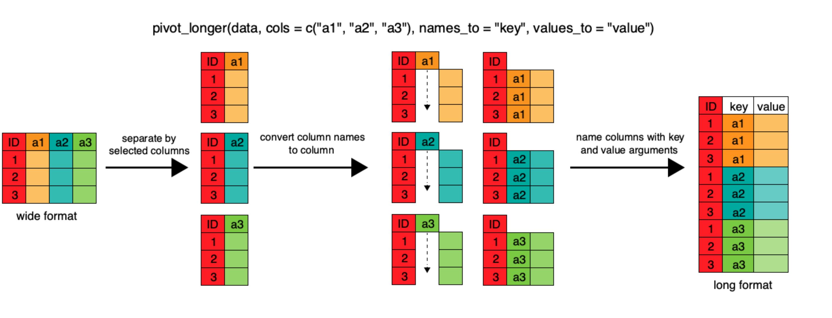
pivot_longer figure
Let’s pretend that we got sent the dataset we just created (wide_survey) and we want to reshape it to be in a long format. We can easily do that using pivot_longer
#cols = columns to be pivoted. Here we want to pivot all the plot_id columns, except the colum "genus"
#names_to = the name of the new column we created from the `cols` argument
#values_to = the name of the new column we will put our values in

surveys_long <- wide_survey %>% pivot_longer(col = -genus, names_to = "plot_id", values_to = "mean_weight")
This data set should look just like surveys_mz. But this one is 240 rows, and surveys_mz is 196 rows. What’s going on?
View(surveys_long)Looks like all the NAs are included in this data set. This is always going to happen when moving between pivot_longer and pivot_wider, but is actually a useful way to balance out a dataset so every replicate has the same composition. Luckily, we now know how to remove the NAs if we want!
surveys_long <- surveys_long %>%
  filter(!is.na(mean_weight)) #now 196 rows
pivot_wider and pivot_longer are both new additions to the tidyverse which means there are some cool new blog posts detailing all their abilities. If you’d like to read more about this group of functions, check out these links:
Challenge
- Use
pivot_wideron thesurveysdata frame withyearas columns,plot_idas rows, and the number of genera per plot as the values. You will need to summarize before reshaping, and use the functionn_distinct()to get the number of unique genera within a particular chunk of data. It’s a powerful function! See?n_distinctfor more. - The
surveysdata set has two measurement columns:hindfoot_lengthandweight. This makes it difficult to do things like look at the relationship between mean values of each measurement per year in different plot types. Let’s walk through a common solution for this type of problem. First, usepivot_longer()to create a dataset where we have a new column calledmeasurementand avaluecolumn that takes on the value of eitherhindfoot_lengthorweight. Hint: You’ll need to specify which columns are being gathered. - With this new data set, calculate the average of each
measurementin eachyearfor each differentplot_type. Thenspread()them into a data set with a column forhindfoot_lengthandweight. Hint: You only need to specify the key and value columns forspread()
ANSWER
## Answer 1
q1 <- surveys %>%
  group_by(plot_id, year) %>%
  summarize(n_genera = n_distinct(genus)) %>%
  pivot_wider(names_from = "year", values_from = "n_genera")

head(q1)
## # A tibble: 6 x 27
## # Groups: plot_id [6]
## plot_id `1977` `1978` `1979` `1980` `1981` `1982` `1983` `1984` `1985`
## <dbl> <int> <int> <int> <int> <int> <int> <int> <int> <int>
## 1 1 2 3 4 7 5 6 7 6 4
## 2 2 6 6 6 8 5 9 9 9 6
## 3 3 5 6 4 6 6 8 10 11 7
## 4 4 4 4 3 4 5 4 6 3 4
## 5 5 4 3 2 5 4 6 7 7 3
## 6 6 3 4 3 4 5 9 9 7 5
## # … with 17 more variables: `1986` <int>, `1987` <int>, `1988` <int>,
## # `1989` <int>, `1990` <int>, `1991` <int>, `1992` <int>, `1993` <int>,
## # `1994` <int>, `1995` <int>, `1996` <int>, `1997` <int>, `1998` <int>,
## # `1999` <int>, `2000` <int>, `2001` <int>, `2002` <int>## Answer 2
q2 <- surveys %>%
pivot_longer(cols = c("hindfoot_length", "weight"), names_to = "measurement_type", values_to = "value")
#cols = columns we want to manipulate
#names_to = name of new column
#values_to = the values we want to fill our new column with (here we already told the function that we were intersted in hindfoot_length and weight, so it will automatically fill our new column, which we named "values", with those numbers.)
## Answer 3
q3 <- q2 %>%
group_by(year, measurement_type, plot_type) %>%
summarize(mean_value = mean(value, na.rm=TRUE)) %>%
pivot_wider(names_from = "measurement_type", values_from = "mean_value")