Using RMarkdown
Ryan Peek
Visualize & Communicate
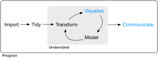
If we consider the data science workflow we showed earlier, we’ve covered most of the steps, save the last few. The excellent R for Data Science online book by Garrett Grolemund & Hadley Wickham gives a nice run down of the various pieces that the last two steps may entail (Visualization and Communication). We’ll use some examples from that book, along with some of additional code you may recognize from previous lessons.
R Markdown
RMarkdown is an excellent tool that is built into RStudio. It provides many options and is a very flexible and powerful platform for authoring HTML, PDF, and MS Word documents, using the Markdown language. RStudio has some excellent resources for this, be sure to visit their site: http://rmarkdown.rstudio.com.
You can use RMarkdown as a digital notebook of all you’ve done or the code you’ve used, or you can write a more formal report that summarizes a project or experiment. This lesson won’t cover everything (not even close!), but it should introduce you to some of the possibilities, and get you comfortable using RMarkdown inside RStudio.
What’s Markdown?
Markdown is plain text shorthand with a simple formatting syntax that can be easily translated or transformed into html formats. RStudio has some great references you can use, go to Help > Markdown Quick Reference, or checkout some of the fancy cheatsheets.
What’s Knitting?
When you open a new .Rmd document, you’ll get a basic template with some demo text and code. If you look for the Knit button at the top of the document, and click the small arrow just to the right of that button, you’ll see a number of options for generating different document formats.
Just to the right of the Knit button, there’s a gear wheel with a small arrow to the right. Click on the small arrow and notice the various output options…these help determine where your content will end up when you Knit, or run chunks of code in your Rmd. We can play with these and determine what is most preferable.
Rmarkdown Components
Code Chunks
The main advantage of using Rmarkdown vs. just markdown is that we can include R code chunks. Take a look at the RMarkdown default, and take a look at the example Rmarkdown file from R for Data Science.
To add a code chunk, we can use the shortcut Ctrl/Cmd + Alt/Option + i:
library(tidyverse)
library(viridis) # let's use some color palette options!
## Loading required package: viridisLite# let's use a new dataset we haven't tried before "storms"
glimpse(storms)## Observations: 10,010
## Variables: 13
## $ name <chr> "Amy", "Amy", "Amy", "Amy", "Amy", "Amy", "Amy", "Am…
## $ year <dbl> 1975, 1975, 1975, 1975, 1975, 1975, 1975, 1975, 1975…
## $ month <dbl> 6, 6, 6, 6, 6, 6, 6, 6, 6, 6, 6, 6, 6, 6, 6, 6, 7, 7…
## $ day <int> 27, 27, 27, 27, 28, 28, 28, 28, 29, 29, 29, 29, 30, …
## $ hour <dbl> 0, 6, 12, 18, 0, 6, 12, 18, 0, 6, 12, 18, 0, 6, 12, …
## $ lat <dbl> 27.5, 28.5, 29.5, 30.5, 31.5, 32.4, 33.3, 34.0, 34.4…
## $ long <dbl> -79.0, -79.0, -79.0, -79.0, -78.8, -78.7, -78.0, -77…
## $ status <chr> "tropical depression", "tropical depression", "tropi…
## $ category <ord> -1, -1, -1, -1, -1, -1, -1, -1, 0, 0, 0, 0, 0, 0, 0,…
## $ wind <int> 25, 25, 25, 25, 25, 25, 25, 30, 35, 40, 45, 50, 50, …
## $ pressure <int> 1013, 1013, 1013, 1013, 1012, 1012, 1011, 1006, 1004…
## $ ts_diameter <dbl> NA, NA, NA, NA, NA, NA, NA, NA, NA, NA, NA, NA, NA, …
## $ hu_diameter <dbl> NA, NA, NA, NA, NA, NA, NA, NA, NA, NA, NA, NA, NA, …ggplot(data=storms) +
geom_jitter(aes(x=as.factor(month), y=pressure, fill=wind),
pch=21, alpha=0.5) +
scale_fill_viridis_c() +
theme_bw() +
labs(title="Hurricane Pressure vs. Month",
subtitle="with Max Win Speed", x="Month")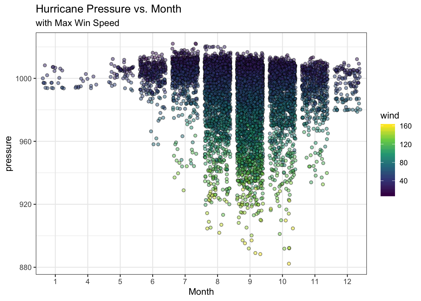
Challenge
There are many options available inside a code chunk. How can we print our code but not evaluate it? Or print our plot but not our code?
Bonus Challenge Question: How can we suppress the package messages that print when we load a package?
Weblinks
You can add links to your Rmd. To do so, there are two options. A full link can be included as is:
Or to try hyperlinking a word or series of words, you can use the following syntax:
[the words you want to hyperlink](the.full.url.here)- So, this is the link to the gapminder csv
Photos/Images
Similarly we can add photos, figures, gifs, embed youtube videos, etc. Really most anything we’d like to include.
For example, to include a figure from our computer, we use:


This works for gifs too!

Or if you want to embed a video, you can use the following code:
<iframe width="480" height="270" src="https://www.youtube.com/embed/7PCQ5vfCsZU" frameborder="0" allow="autoplay; encrypted-media" allowfullscreen></iframe>
Equations & Formulas
Using a language called LaTeX we can embed formulas into our RMarkdown. You can do equations inline or as stand-alone formulas. The syntax requires a $ on either side for inline, for example the following:
This summation expression $\sum_{i=y}^n X_i$ appears inline.
Will render like this:
- This summation expression \(\sum_{i=y}^n X_i\) appears inline.
To make a formula, you can use the $$ in front and at the end.
\[ \Sigma = \frac{\theta + y_{i}}{x + ab} \]
Tables
Tables can be created as well, there are many flavors and packages you can use. This is just a quick sample of some of the options:
kable
This is part of the knitr package. It’s handy and makes nice tables quickly:
library(knitr)
kable(head(storms), caption = "Table with kable")| name | year | month | day | hour | lat | long | status | category | wind | pressure | ts_diameter | hu_diameter |
|---|---|---|---|---|---|---|---|---|---|---|---|---|
| Amy | 1975 | 6 | 27 | 0 | 27.5 | -79.0 | tropical depression | -1 | 25 | 1013 | NA | NA |
| Amy | 1975 | 6 | 27 | 6 | 28.5 | -79.0 | tropical depression | -1 | 25 | 1013 | NA | NA |
| Amy | 1975 | 6 | 27 | 12 | 29.5 | -79.0 | tropical depression | -1 | 25 | 1013 | NA | NA |
| Amy | 1975 | 6 | 27 | 18 | 30.5 | -79.0 | tropical depression | -1 | 25 | 1013 | NA | NA |
| Amy | 1975 | 6 | 28 | 0 | 31.5 | -78.8 | tropical depression | -1 | 25 | 1012 | NA | NA |
| Amy | 1975 | 6 | 28 | 6 | 32.4 | -78.7 | tropical depression | -1 | 25 | 1012 | NA | NA |
htmltable
htmlTable::htmlTable(head(storms))| name | year | month | day | hour | lat | long | status | category | wind | pressure | ts_diameter | hu_diameter | |
|---|---|---|---|---|---|---|---|---|---|---|---|---|---|
| 1 | Amy | 1975 | 6 | 27 | 0 | 27.5 | -79 | tropical depression | -1 | 25 | 1013 | ||
| 2 | Amy | 1975 | 6 | 27 | 6 | 28.5 | -79 | tropical depression | -1 | 25 | 1013 | ||
| 3 | Amy | 1975 | 6 | 27 | 12 | 29.5 | -79 | tropical depression | -1 | 25 | 1013 | ||
| 4 | Amy | 1975 | 6 | 27 | 18 | 30.5 | -79 | tropical depression | -1 | 25 | 1013 | ||
| 5 | Amy | 1975 | 6 | 28 | 0 | 31.5 | -78.8 | tropical depression | -1 | 25 | 1012 | ||
| 6 | Amy | 1975 | 6 | 28 | 6 | 32.4 | -78.7 | tropical depression | -1 | 25 | 1012 |
DT(interactive tables)
DT::datatable(storms)## Warning in instance$preRenderHook(instance): It seems your data is too
## big for client-side DataTables. You may consider server-side processing:
## https://rstudio.github.io/DT/server.htmlAdditional packages for creating tables include stargazer and xtable.
Footnotes
- We can include footnotes as well1
Interactivity
There are many great interactive options available using RMarkdown and R code. Perhaps my most favorite is plotly. You can wrap most any ggplot with ggplotly() and make it interactive.
# library(plotly)

plotly::ggplotly(
  ggplot(data=storms) +
    geom_jitter(aes(x=as.factor(month), y=pressure, color=wind),
                alpha=0.5) +
    scale_color_viridis_c() +
    theme_bw() +
    labs(title="Hurricane Pressure vs. Month",
         subtitle="with Max Win Speed", x="Month")
)
Other options include a great mapping package called mapview. Don’t worry too much about the code here, but just be aware these are options for you to look into in the future.
library(leaflet)

# filter data down
storms <- filter(storms, year > 2006)

# set up a color palette:
pal <- colorNumeric(
  palette = "RdYlBu",
  domain = storms$wind)

# make a map
m <- leaflet() %>% addTiles() %>%
  addProviderTiles("Esri.WorldImagery", group = "ESRI Aerial") %>%
  addProviderTiles("Esri.WorldTopoMap", group = "Topo") %>%

# proposed sites
  addCircleMarkers(data=storms, group="Storms",
                   lng= ~long, lat= ~lat,
                   stroke=TRUE, weight=0.6, radius=4,
                   fillOpacity = 0.5, color=~pal(wind)) %>%

  # add controls for basemaps and data
  addLayersControl(
    baseGroups = c("ESRI Aerial", "Topo"),
    overlayGroups = c("Storms"),
    options = layersControlOptions(collapsed = T))

m
Citations
There are also options for citations…you can add a .bib file in your YAML header. See RStudio’s demo for a short overview.
This lesson was contributed by Ryan Peek.
A footnote here for fun↩