Dates & Times in R
Working with datetimes and lubridate
Learning Objectives
- Learn the basic date/datetime types in R
- Gain familiarity with converting dates and timezones
- Learn how to use the
lubridatepackage - Tips and tricks about management of datetime data
Date-Times in R
We have learned about different data type classes in previous lessons. Some common data classes we have examined before include character, factor, and numeric. But R also recognizes a data class called “Dates”. Having your date data in the “Dates” data class is very useful, as you can then do things like calculate time between two events, transform the dates into different formats, and plot temporal data easily. In this lesson, we are going to introduce how base R deals with dates (POSIXct or POSITlt), but we are going to spend the majority of our lesson on the package lubridate. lubridate is a great package that makes it much easier to work with dates and times in R.
Date-Time Classes in Base R
Importantly, there are 3 basic time classes in R:
Dates(just dates, i.e., 2012-02-10)POSIXct(“ct” == calendar time, best class for dates with times)POSIXlt(“lt” == local time, enables easy extraction of specific components of a time, however, remember that POXIXlt objects are lists)
Unfortunately converting dates & times in R into formats that are computer readable can be frustrating, mainly because there is very little consistency. In particular, if you are importing things from Excel, keep in mind dates can get especially weird1, depending on the operating system you are working on, the format of your data, etc.
1 For example Excel stores dates as a number representing days since 1900-Jan-0, plus a fractional portion of a 24 hour day (serial-time), but in OSX (Mac), it is 1904-Jan-0.
Dates
The Date class in R can easily be converted or operated on numerically, depending on the interest. Let’s make a string of dates to use for our example:
sample_dates_1 <- c("2018-02-01", "2018-03-21", "2018-10-05", "2019-01-01", "2019-02-18")
#notice we have dates across two years here
What is the class that R classifies this data as?
R classifies our sample_dates_1 data as character data. Let’s transform it into Dates. Notice that our sample_dates_1 is in a nice format: YYYY-MM-DD. This is the format necessary for the function as.Date.
sample_dates_1 <- as.Date(sample_dates_1)What happens with different orders…say MM-DD-YYYY?
# Some sample dates:

sample_dates_2 <- c("02-01-2018", "03-21-2018", "10-05-2018", "01-01-2019", "02-18-2019")

sample_dates_3 <-as.Date(sample_dates_2) # well that doesn't work
The reason this doesn’t work is because the computer expects one thing, but is getting something else. Remember, write code you can read and your computer can understand. So we need to give some more information here so R will interpret our data correctly.
# Some sample dates:
sample_dates_2 <- c("02-01-2018", "03-21-2018", "10-05-2018", "01-01-2019", "02-18-2019")

sample_dates_3<- as.Date(sample_dates_2, format = "%m-%d-%Y" ) # date code preceded by "%"
To see a list of the date-time format codes in R, check out this page and table, or you can use: ?(strptime)
The nice thing is this method works well with pretty much any format, you just need to provide the associated codes and structure:
as.Date("2016/01/01", format="%Y/%m/%d")=2016-01-01as.Date("05A21A2011", format="%mA%dA%Y")=2011-05-21
Challenge
Format this date with the as.Date function: Jul 04, 2019
ANSWER
as.Date("Jul 04, 2019", format = "%b%d,%Y")## [1] "2019-07-04"Working with Times in Base R
When working with times, the best class to use in base R is POSIXct.
tm1 <- as.POSIXct("2016-07-24 23:55:26")
tm1
## [1] "2016-07-24 23:55:26 PDT"tm2 <- as.POSIXct("25072016 08:32:07", format = "%d%m%Y %H:%M:%S")
tm2## [1] "2016-07-25 08:32:07 PDT"#Notice how POSIXct automatically uses the timezone your computer is set to. What if we collected this data in a different timezone?
# specify the time zone:
tm3 <- as.POSIXct("2010-12-01 11:42:03", tz = "GMT")
tm3## [1] "2010-12-01 11:42:03 GMT"The lubridate Package
The lubridate package will handle 90% of the date & datetime issues you need to deal with. It is fast, much easier to work with, and we recommend using it wherever possible. Do keep in mind sometimes you need to fall back on the base R functions (i.e., as.Date()), which is why having a basic understanding of theses functions and their use is important.
To use lubridate we will first need to install and load the package.
#install.packages("lubridate")

library(lubridate)
lubridate has lots of handy functions for converting between date and time formats, and even timezones.
Let’s take a look at our sample_dates_1 data again.
sample_dates_1 <- c("2018-02-01", "2018-03-21", "2018-10-05", "2019-01-01", "2019-02-18")Once again, R reads this in a character data.
Lubridate uses functions that looks like ymd or mdy to transform data into the class “Date”. Our sample_dates_1 data is formatted like Year, Month, Day, so we would use the lubridate function ymd (y = year, m = month, d = day).
sample_dates_lub <- ymd(sample_dates_1)What about that messier sample_dates_2 data? Remember R wants dates to be in the format YYYY-MM-DD.
sample_dates_2 <- c("2-01-2018", "3-21-2018", "10-05-18", "01-01-2019", "02-18-2019")
#notice that some numbers for years and months are missing

sample_dates_lub2 <- mdy(sample_dates_2) #lubridate can handle it!
All sorts of date formats can easily be transformed using lubridate:
lubridate::ymd("2016/01/01")=2016-01-01lubridate::ymd("2011-03-19")=2011-03-19lubridate::mdy("Feb 19, 2011")=2011-02-19lubridate::dmy("22051997")=1997-05-22
Using lubridate for Time and Timezones
lubridate has very similar functions to handle data with Times and Timezones. To the ymd function, add _hms or _hm (h= hours, m= minute, s= seconds) and a tz argument. lubridate will default to the POSIXct format.
- Example 1:
lubridate::ymd_hm("2016-01-01 12:00", tz="America/Los_Angeles")= 2016-01-01 12:00:00 - Example 2 (24 hr time):
lubridate::ymd_hm("2016/04/05 14:47", tz="America/Los_Angeles")= 2016-04-05 14:47:00 - Example 3 (12 hr time but converts to 24):
lubridate::ymd_hms("2016/04/05 4:47:21 PM", tz="America/Los_Angeles")= 2016-04-05 16:47:21
Lubridate Tips
For lubridate to work, you need the column datatype to be character or factor. The readr package (from the tidyverse) is smart and will try to guess for you. Problem is, it might convert your data for you without the settings (in this case the proper timezone). So here are few ways to work around this.
library(lubridate)
library(dplyr)
library(readr)

# read in some data and skip header lines
nfy1 <- read_csv("data/2015_NFY_solinst.csv", skip = 12)
head(nfy1) #R tried to guess for you that the first column was a date and the second a time
## # A tibble: 6 x 5
## Date Time ms Level Temperature
## <date> <time> <dbl> <dbl> <dbl>
## 1 2015-05-22 14:00 0 -8.68 0
## 2 2015-05-22 14:15 0 -8.29 0
## 3 2015-05-22 14:30 0 -8.29 0
## 4 2015-05-22 14:45 0 -8.29 0
## 5 2015-05-22 15:00 0 -8.30 0
## 6 2015-05-22 15:15 0 -8.29 0# import raw dataset & specify column types
nfy2 <- read_csv("data/2015_NFY_solinst.csv", col_types = "ccidd", skip=12)
glimpse(nfy1) # notice the data types in the Date.Time and datetime cols## Observations: 7,764
## Variables: 5
## $ Date <date> 2015-05-22, 2015-05-22, 2015-05-22, 2015-05-22, 201…
## $ Time <time> 14:00:00, 14:15:00, 14:30:00, 14:45:00, 15:00:00, 1…
## $ ms <dbl> 0, 0, 0, 0, 0, 0, 0, 0, 0, 0, 0, 0, 0, 0, 0, 0, 0, 0…
## $ Level <dbl> -8.6834, -8.2928, -8.2914, -8.2901, -8.2955, -8.2935…
## $ Temperature <dbl> 0, 0, 0, 0, 0, 0, 0, 0, 0, 0, 0, 0, 0, 0, 0, 0, 0, 0…glimpse(nfy2)## Observations: 7,764
## Variables: 5
## $ Date <chr> "2015/05/22", "2015/05/22", "2015/05/22", "2015/05/2…
## $ Time <chr> "14:00:00", "14:15:00", "14:30:00", "14:45:00", "15:…
## $ ms <int> 0, 0, 0, 0, 0, 0, 0, 0, 0, 0, 0, 0, 0, 0, 0, 0, 0, 0…
## $ Level <dbl> -8.6834, -8.2928, -8.2914, -8.2901, -8.2955, -8.2935…
## $ Temperature <dbl> 0, 0, 0, 0, 0, 0, 0, 0, 0, 0, 0, 0, 0, 0, 0, 0, 0, 0…# make a datetime col:
nfy2$datetime <- paste(nfy2$Date, " ", nfy2$Time, sep = "")
glimpse(nfy2) #notice the datetime column is classifed as character## Observations: 7,764
## Variables: 6
## $ Date <chr> "2015/05/22", "2015/05/22", "2015/05/22", "2015/05/2…
## $ Time <chr> "14:00:00", "14:15:00", "14:30:00", "14:45:00", "15:…
## $ ms <int> 0, 0, 0, 0, 0, 0, 0, 0, 0, 0, 0, 0, 0, 0, 0, 0, 0, 0…
## $ Level <dbl> -8.6834, -8.2928, -8.2914, -8.2901, -8.2955, -8.2935…
## $ Temperature <dbl> 0, 0, 0, 0, 0, 0, 0, 0, 0, 0, 0, 0, 0, 0, 0, 0, 0, 0…
## $ datetime <chr> "2015/05/22 14:00:00", "2015/05/22 14:15:00", "2015/…# convert Date Time to POSIXct in local timezone using lubridate
nfy2$datetime_test <- as_datetime(nfy2$datetime,
tz="America/Los_Angeles")
# OR convert using the ymd_functions
nfy2$datetime_test2 <- ymd_hms(nfy2$datetime, tz="America/Los_Angeles")
# OR wrap in as.character()
nfy1$datetime <- ymd_hms(as.character(paste0(nfy1$Date," ", nfy1$Time)), tz="America/Los_Angeles")
tz(nfy1$datetime)## [1] "America/Los_Angeles"Example 1: Mauna Loa Meteorological Data
So, now that we have a decent idea how to format these things, let’s look at some real data, try to format and plot. Let’s use the Mauna Loa meteorological data, collected every minute for the year 2001. This dataset has 459,769 observations for 9 different metrics of wind, humidity, barometric pressure, air temperature, and precipitation. Download this dataset here. Save it to your data/ folder. Alternatively, you can find it on the R-DAVIS website in the Resources->Datasets tab.
load("data/mauna_loa_met_2001_minute.rda")

# just renaming the object loaded by the RDA file
mloa <- mloa_2001

library(lubridate, warn.conflicts = F)
library(dplyr, warn.conflicts = F)

summary(mloa)
## filename siteID year month
## Length:459769 MLO:459769 Min. :2001 Min. : 1.000
## Class :character 1st Qu.:2001 1st Qu.: 3.000
## Mode :character Median :2001 Median : 6.000
## Mean :2001 Mean : 6.474
## 3rd Qu.:2001 3rd Qu.:10.000
## Max. :2001 Max. :12.000
## day hour24 min windDir
## Min. : 1.00 Min. : 0.00 Min. : 0.00 Min. :-999.0
## 1st Qu.: 8.00 1st Qu.: 5.00 1st Qu.:15.00 1st Qu.: 115.0
## Median :15.00 Median :11.00 Median :30.00 Median : 156.0
## Mean :15.44 Mean :11.43 Mean :29.51 Mean : 144.5
## 3rd Qu.:22.00 3rd Qu.:18.00 3rd Qu.:45.00 3rd Qu.: 236.0
## Max. :31.00 Max. :23.00 Max. :59.00 Max. : 360.0
## windSpeed_m_s windSteady baro_hPa temp_C_2m
## Min. :-99.900 Min. :-9 Min. :-999.9 Min. :-999.900
## 1st Qu.: 1.900 1st Qu.:-9 1st Qu.:-999.9 1st Qu.: 4.400
## Median : 3.500 Median :-9 Median :-999.9 Median : 6.900
## Mean : 1.229 Mean :-9 Mean :-999.9 Mean : 4.747
## 3rd Qu.: 5.900 3rd Qu.:-9 3rd Qu.:-999.9 3rd Qu.: 9.400
## Max. : 20.500 Max. :-9 Max. :-999.9 Max. : 18.900
## temp_C_10m temp_C_towertop rel_humid precip_intens_mm_hr
## Min. :-999.90 Min. :-999.900 Min. :-99.00 Min. :-99.0000
## 1st Qu.: 4.90 1st Qu.: 5.600 1st Qu.: 14.00 1st Qu.: 0.0000
## Median : 6.90 Median : 7.200 Median : 28.00 Median : 0.0000
## Mean : -46.69 Mean : 1.539 Mean : 31.82 Mean : -0.8066
## 3rd Qu.: 8.60 3rd Qu.: 8.800 3rd Qu.: 57.00 3rd Qu.: 0.0000
## Max. : 16.90 Max. : 16.200 Max. :138.00 Max. : 60.0000names(mloa)## [1] "filename" "siteID" "year"
## [4] "month" "day" "hour24"
## [7] "min" "windDir" "windSpeed_m_s"
## [10] "windSteady" "baro_hPa" "temp_C_2m"
## [13] "temp_C_10m" "temp_C_towertop" "rel_humid"
## [16] "precip_intens_mm_hr"One of the important components to consider is each of the datetime columns has been separated…so how do we get them into one column so we can format it as a datetime? The answer is the paste function.
paste()allows pasting text or vectors (& columns) by a given separator that you specifypaste0()is the same thing, but defaults to using a,as the separator.
# we need to make a datetime column...let's use paste
mloa$datetime <- paste0(mloa$year,"-", mloa$month, "-", mloa$day," ", mloa$hour24, ":", mloa$min) # this makes a character column

head(mloa$datetime) # character vector but not POSIXct yet
## [1] "2001-1-1 0:0" "2001-1-1 0:1" "2001-1-1 0:2" "2001-1-1 0:3"
## [5] "2001-1-1 0:4" "2001-1-1 0:5"# we can nest this within a lubridate function to convert directly to POSIXct
mloa$datetime <- ymd_hm(mloa$datetime, tz="Pacific/Honolulu")
# OR all in one step
mloa$datetime <- ymd_hm(paste0(mloa$year,"-", mloa$month, "-", mloa$day," ", mloa$hour24, ":", mloa$min), tz = "Pacific/Honolulu")
summary(mloa) # notice a new column called "datetime"## filename siteID year month
## Length:459769 MLO:459769 Min. :2001 Min. : 1.000
## Class :character 1st Qu.:2001 1st Qu.: 3.000
## Mode :character Median :2001 Median : 6.000
## Mean :2001 Mean : 6.474
## 3rd Qu.:2001 3rd Qu.:10.000
## Max. :2001 Max. :12.000
## day hour24 min windDir
## Min. : 1.00 Min. : 0.00 Min. : 0.00 Min. :-999.0
## 1st Qu.: 8.00 1st Qu.: 5.00 1st Qu.:15.00 1st Qu.: 115.0
## Median :15.00 Median :11.00 Median :30.00 Median : 156.0
## Mean :15.44 Mean :11.43 Mean :29.51 Mean : 144.5
## 3rd Qu.:22.00 3rd Qu.:18.00 3rd Qu.:45.00 3rd Qu.: 236.0
## Max. :31.00 Max. :23.00 Max. :59.00 Max. : 360.0
## windSpeed_m_s windSteady baro_hPa temp_C_2m
## Min. :-99.900 Min. :-9 Min. :-999.9 Min. :-999.900
## 1st Qu.: 1.900 1st Qu.:-9 1st Qu.:-999.9 1st Qu.: 4.400
## Median : 3.500 Median :-9 Median :-999.9 Median : 6.900
## Mean : 1.229 Mean :-9 Mean :-999.9 Mean : 4.747
## 3rd Qu.: 5.900 3rd Qu.:-9 3rd Qu.:-999.9 3rd Qu.: 9.400
## Max. : 20.500 Max. :-9 Max. :-999.9 Max. : 18.900
## temp_C_10m temp_C_towertop rel_humid precip_intens_mm_hr
## Min. :-999.90 Min. :-999.900 Min. :-99.00 Min. :-99.0000
## 1st Qu.: 4.90 1st Qu.: 5.600 1st Qu.: 14.00 1st Qu.: 0.0000
## Median : 6.90 Median : 7.200 Median : 28.00 Median : 0.0000
## Mean : -46.69 Mean : 1.539 Mean : 31.82 Mean : -0.8066
## 3rd Qu.: 8.60 3rd Qu.: 8.800 3rd Qu.: 57.00 3rd Qu.: 0.0000
## Max. : 16.90 Max. : 16.200 Max. :138.00 Max. : 60.0000
## datetime
## Min. :2001-01-01 00:00:00
## 1st Qu.:2001-03-29 06:57:00
## Median :2001-06-24 06:13:00
## Mean :2001-06-30 15:28:42
## 3rd Qu.:2001-10-07 00:34:00
## Max. :2001-12-31 23:59:00head(mloa$datetime) # in POSIXct## [1] "2001-01-01 00:00:00 HST" "2001-01-01 00:01:00 HST"
## [3] "2001-01-01 00:02:00 HST" "2001-01-01 00:03:00 HST"
## [5] "2001-01-01 00:04:00 HST" "2001-01-01 00:05:00 HST"Challenge with dplyr and ggplot
Let’s plot some of the Mauna Loa data we just downloaded. First, removed the NAs (here designated with -99.9 and -999.9) in rel_humid, temp_C_2m, and windSpeed_m_s. Next, use dplyr to calculate the mean monthly temperature using the temp_C_2m column and the datetime column. (*HINT: Look at the lubridate function called month()). Finally, make a ggplot of the mean monthly temperature.
EXTRA CHALLENGE: Make a ggplot of the average hourly temperature during the month of July
ANSWER
library(dplyr)
library(ggplot2)
library(lubridate)

# clean up the NA data (NA's are = -99 or -999 depending on data col)
df <- mloa %>%
  filter(!rel_humid == -99, !temp_C_2m == -999.9, !windSpeed_m_s == -99.9) %>% #removing NAs
  mutate(mon=month(datetime, label = TRUE, abbr=TRUE)) #making new column where each month is named

df2 <- df %>%
  group_by(mon) %>%
  summarize(avg_temp_2m = mean(temp_C_2m)) #average monthly temperature

df2 %>%
  ggplot() +
  geom_point(aes(x=mon, y=avg_temp_2m), color="darkblue", size= 3)+
  ylab("Avg Monthly Temperature (C)") + xlab("Month")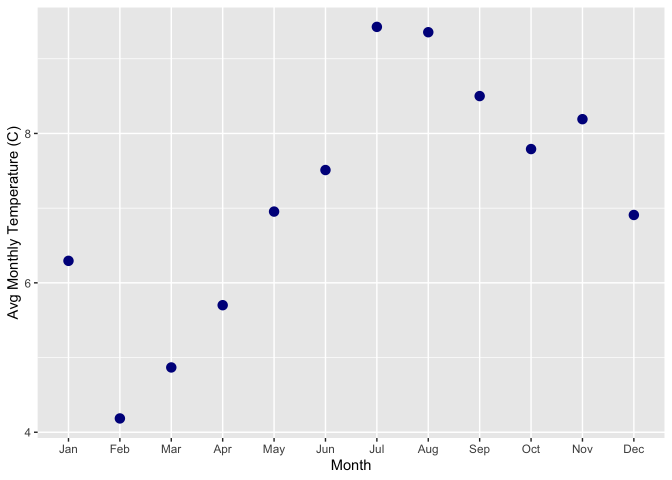
This lesson was contributed by Ryan Peek and Martha Zillig.