Data Import and Export
Learning objectives
- Get comfortable importing different kinds of data
- Understand the concept of “tidy data”
Reading csv data
Data come in many forms, and we need to be able to load them in R. For our own use and with others who use R, there are R-specific data structures we can use, such as the .rda (.RDATA), or the .rds file-types. We’ll talk about those in more detail later. However, we need to be able to work with more general data types too. Comma-separated value (.csv) tables are perhaps the most universal data structure.
This species dataset provides genus and species information for animals caught during a trapping survey. I downloaded it and put it in the data directory of my project. Click on the link and download the file.
Review: What’s the main difference between read.csv and read_csv?
Answer: stringsAsFactors=FALSE
By default, when building or importing a data frame, the columns that contain characters (i.e., text) are coerced (=converted) into the factor data type when we use the read.csv. Depending on what you want to do with the data, you may want to keep these columns as character. To do so, read.csv() and read.table() have an argument called stringsAsFactors which can be set to FALSE.
When we use the tidyverse read_csv all character columns are automatically kept as characters, NOT coherced into factors.
Let’s look at the same data file read in with read.csv and read_csv
surveys_dot <- read.csv('data/combined.csv')

surveys_underscore <- read_csv("data/combined.csv")
## Parsed with column specification:
## cols(
## record_id = col_double(),
## month = col_double(),
## day = col_double(),
## year = col_double(),
## plot_id = col_double(),
## species_id = col_character(),
## sex = col_character(),
## hindfoot_length = col_double(),
## weight = col_double(),
## genus = col_character(),
## species = col_character(),
## taxa = col_character(),
## plot_type = col_character()
## )#using stringAsfactor
surveys_dot2 <- read.csv("data/combined.csv", stringsAsFactors = FALSE)
#can use as.character or as.factor to change single column types Advanced challenge
Suppose you get a .csv file from a colleague in Europe. Because they use , (comma) as a decimal separator, they use ; (semi-colons) to separate fields.
- How can you read it into R? Feel free to use the web and/or R’s helpfiles.
Reading messier data
Sometimes data can be a bit trickier to read because it isn’t in tidy format. If it is close to being tidy, we may be able add some more arguments to the read_csv() call to to help R interpret how the file should be read.
Use this link to download this “wide” dataset and inspect it with a spreadsheet program. Why isn’t it tidy?
Try using the read.csv() function on the file.
read_csv("data/wide_eg.csv")We need to tell R to skip 2 rows!
read_csv("data/wide_eg.csv", skip = 2)We can use the read_csv() function to read files directly from a website.
read_csv("https://mikoontz.github.io/data-carpentry-week/data/wide_eg.csv", skip = 2)Exporting data
Now that you have learned how to use dplyr to extract information from or summarize your raw data, you may want to export these new datasets to share them with your collaborators or for archival.
Similar to the read_csv() function used for reading CSV files into R, there is a write_csv() function that generates CSV files from data frames.
Before using write_csv(), we are going to create a new folder, data_output, in our working directory that will store this generated dataset. We don’t want to write generated datasets in the same directory as our raw data. It’s good practice to keep them separate. The data folder should only contain the raw, unaltered data, and should be left alone to make sure we don’t delete or modify it. In contrast, our script will generate the contents of the data_output directory, so even if the files it contains are deleted, we can always re-generate them.
- Type in
write_and hit TAB. Scroll down and take a look at the many options that exist for writing out data in R. Use the F1 key on any of these options to read more about how to use it.
Using save and load
We’ve seen how to save out specific data types in R. One additional option is you can save anything in your workspace or working “environment”. You can save a single object, or multiple objects together. This is best done using the .rda file type. The .Rda file type is a great way to save objects from R that you have already tidied or modeled, and you want to maintain the structure and format of the data. Because these are native “R” file types, they can be read back in and will appear exactly as when you saved them.
Let’s assume we have the “surveys_underscore” object and the “surveys_dot2” objects in our environment, and we want save them both in one file. We’ll use save() and the .rda filetype.
save(surveys_underscore, surveys_dot2, file = "data_output/surveys_types.rda")To re-load these back into R, we use the load function.
load("data_output/surveys_types.rda").rds vs. .rda
Why use one vs. the other? What do these file types provide that a simple csv doesn’t provide?
Short answer is they maintain not only the structure, but also the format and data types within your data sets. However it appears in your environment in R is exactly how it will be saved (with save()), and then read back in (with load() or readRDS. This can save time and code, once you have your data in a format/shape you are happy with. An added bonus is the format (rda and rds) are both highly compressed, and can save significant space on your hard drive.
The main differences between the two:
.rdaallows saving multiple objects together in one file, or one single object.rdscan only save file/object
For example, let’s use the surveys dataset we loaded earlier and save a few rda and rds files.
library(dplyr)

# load data
surveys <- read_csv('data/combined.csv') # the combined.csv is 3.1 MB in size

# filter to years > 2000 and only rodents
rodents2001 <- surveys %>% filter(year > 2000 & taxa == "Rodent")

# filter to only birds
birds <- surveys %>% filter(taxa=="Bird")

# RDA files: now we can save all these objects together:
save(surveys, rodents2001, birds, file = "data/example.rda") # this file is 245 kb (0.2 MB)

# RDS files: this can only be one file:
saveRDS(rodents2001, file = "data/rodents2001.rds")

# to load an rds file back in:
any_name_i_choose <- readRDS(file = "data/rodents2001.rds")

# but won't work with rda
nope <- readRDS(file = "data/example.rda")

# same with trying to assign a name to an rda file on load
doublenope <- load(file = "data/example.rda") # wait ...check out "doublenope"

doublenope # created a character vector of the objects...but didn't assign any to the name nope

# [1] "surveys"     "rodents2001" "birds"
One extremely time-saving use of .rds files is when you’ve fit a large statistical model that gets saved as a model object. For example, the brms and lme4 packages used for multi-level models will return large model objects that contain lots of information about the model. Some models can take hours, days, even weeks to finish fitting, so it can be useful to save a fully fitted model object as a .rds file. You can then load that model object back into R and work with it however you want.
Saving Figures and Plots
A plot you created with ggplot or another plotting package can be saved as .JPEGS (or .tiff, .img, etc) onto you. For any ggplot objects, we reccomend using ggsave.
Let’s start by making a plot together with our survey data using only data that is for Rodents in years after 2000:
# load data
surveys <- read_csv('data/combined.csv') # the combined.csv is 3.1 MB in size

# filter to years > 2000 and only rodents
rodents2001 <- surveys %>% filter(year > 2000 & taxa == "Rodent")

rodents2001 %>% ggplot()+
        geom_point(aes(x=hindfoot_length, y = weight, color = sex))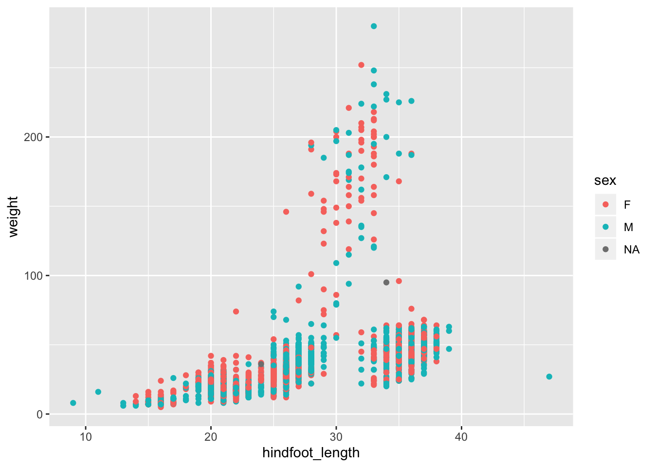
ggsave allows us to easily save this plot. First, let’s create a new folder in this project called figures. Let’s save all the figures we create to that folder. ggsave will default to saving the last plot you created, however, we think it is always a good idea to specify exactly which plot you want saved. To do that, we have to save our plot as an object.
#saving plot as an object
rodent_plot <- rodents2001 %>% ggplot()+
        geom_point(aes(x=hindfoot_length, y = weight, color = sex))

ggsave("figures/rodent1.png", rodent_plot)
With ggsave you can save images as
- .png, .jpeg, .tiff, .pdf, .bmp, or .svg
Other arguments of ggsave
scalecan scale the image (multiplicative scaling factor)widthandheightlet you specify the size of the image inunitsthat you specifydpican change the quality of the image; for publication graphs we suggest over 700 dpi
ggsave("figures/rodent2.png", rodent_plot, width = 4, height = 3, units = "in", dpi = 500)Excel & GoogleSheets
readxl(Part oftidyverse)- Jenny Bryan’s
googlesheetsorgoogledrivepackages
Other File Types
- Using the
foreignpackage - reading in
.dbf, Stata, SAS, SPSS,.shp,.netcdf,raster,.kml,gpx,xml,geojson,json, etc….
rio Package
One other data import/export package to check out is called rio. It uses two main functions: import and export, and it automatically detects the file extension you’re using, then picks the fastest function out of a bunch of different specialized packages. It can streamline your data import/export and give you more consistent data frames when you’re working with lots of different file types.
#install.packages("rio")
library(rio)
export(mtcars, "data/mtcars.csv")
export(mtcars, "data/mtcars.rds")
export(mtcars, "data/mtcars.tsv")
You can read more about rio on its Github page.
This lesson is adapted from the Software Carpentry: R for Reproducible Scientific Analysis Vectors and Data Frames materials and the Data Carpentry: R for Data Analysis and Visualization of Ecological Data Exporting Data materials.